Agentic Retrieval: The Complete Guide from Document Ingestion to Compiled Knowledge
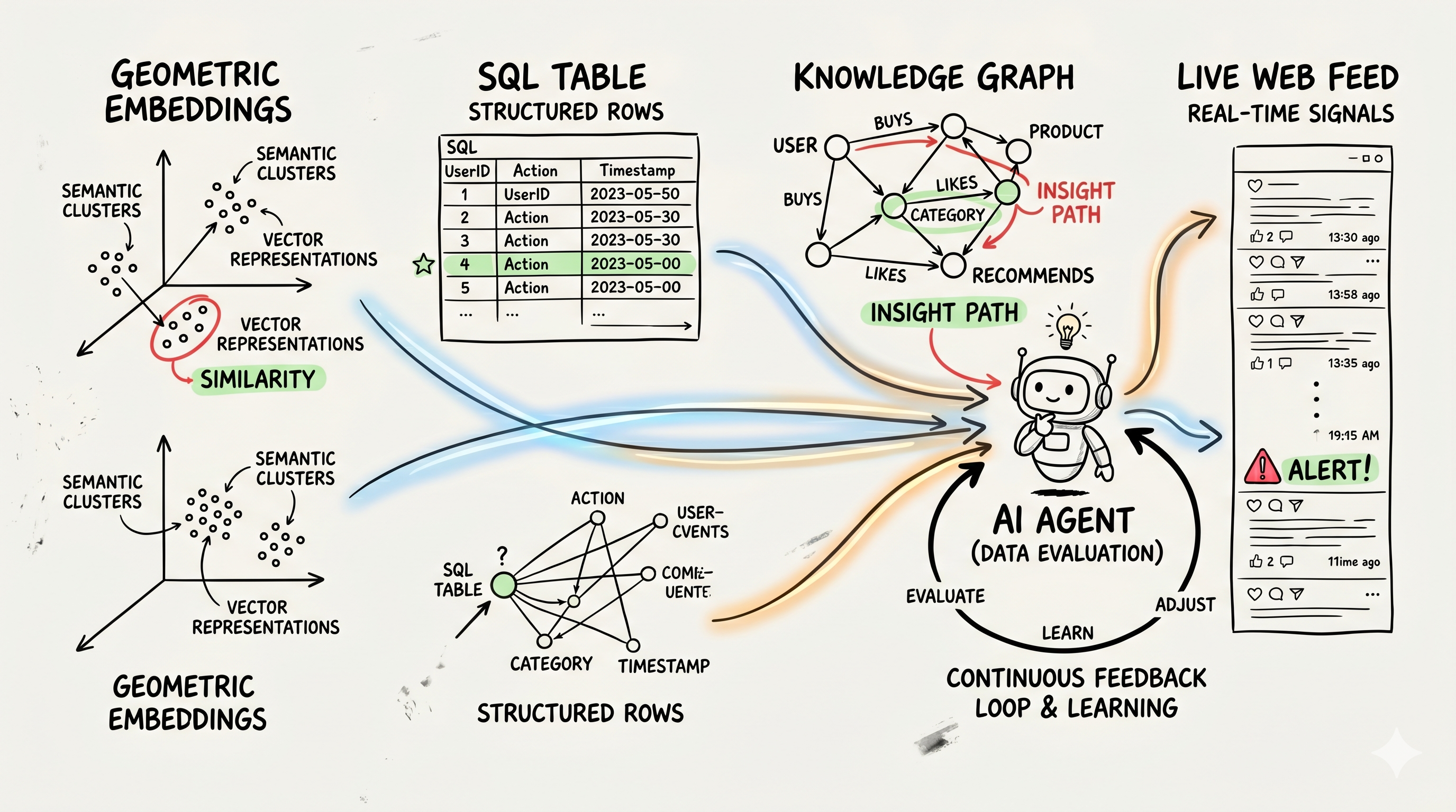
Naive RAG fails roughly 40% of the time at retrieval. Not because the LLM is bad — because what you hand it is bad. Wrong chunks, missing context, no awareness of what it doesn't know. Agentic retrieval fixes the retrieval layer, not the generation layer.
This guide covers the entire pipeline: from ingesting a raw PDF to deploying an agent that queries vector stores, SQL databases, knowledge graphs, and pre-computed summaries — and knows which one to use for each question.
How to read this guide:
- Building your first RAG system? Read the ingestion sections in order, stop at "Re-ranking", ship that, then come back
- Already running naive RAG? Start at "From Naive to Agentic Retrieval"
- Deciding between SQL / graph / GraphRAG? Jump to "Structured & Relational Retrieval: Which One?"
- Prerequisites: working Python; no prior RAG experience needed — every concept is introduced before it's used
A note on the code: samples are condensed for reading. Two habits production code needs that the short samples skip: select the text block by type (
next(b.text for b in response.content if b.type == "text")) rather than indexingcontent[0]— Claude responses can also contain thinking and tool-use blocks — and pin your library versions, since the RAG ecosystem moves fast (version notes are flagged inline where they bite).
Agentic Retrieval
What "Agentic" Actually Means
Traditional RAG is a pipeline: embed the query, find the nearest vectors, stuff them in the prompt, call the LLM. It runs once, retrieves once, generates once. No judgment, no retries, no awareness of what was missed.
Agentic retrieval is a loop. The agent plans which retrieval strategy to use, executes it, evaluates the results, decides whether they're sufficient, and iterates. It's the difference between a researcher who runs one search and accepts whatever shows up versus one who follows citations, checks multiple sources, and reformulates the question when the first search comes up dry.
Naive RAG:     query → embed → ANN search → top-k → LLM
                                                     ↑ done

Agentic RAG:   query → plan retrieval strategy
                     → execute (vector / SQL / graph / hybrid)
                     → evaluate: is this sufficient?
                     → if not: reformulate, query again
                     → synthesize across results
                     → LLM
The Retrieval Spectrum
There are five maturity levels. Most production systems today live at level 2 and pay the price.
| Level | Name | What It Does | Failure Mode |
|---|---|---|---|
| 1 | Keyword Search | BM25 / TF-IDF | Misses paraphrase, synonyms |
| 2 | Naive Vector RAG | Single dense search | Misses exact terms, no iteration |
| 3 | Hybrid RAG | Dense + sparse + reranking | Still single-shot, no reasoning |
| 4 | Agentic RAG | Multi-step, multi-source, evaluated | Higher latency and cost |
| 5 | Compiled Knowledge | Pre-reasoned, structured index | High indexing cost, updates complex |
Start at level 3 in production. Graduate to 4 when your queries require multi-hop reasoning. Level 5 is for domains where the knowledge is stable enough to justify pre-computation.
Which Technique for Which Query
This guide covers a dozen retrieval techniques. Before the deep dives, here's the map — match the shape of the question and the shape of the data to the technique that answers it.
| Question / data shape | Example | Reach for | Why |
|---|---|---|---|
| Conceptual, paraphrased | "What's our refund policy?" | Dense vector | Meaning matches without shared words |
| Exact term, code, ID, SKU | "Error E-2049", part AIS-2026 | Sparse (BM25/SPLADE) | Embeddings blur exact strings |
| Mixed concept + term | "Fix the pgvector timeout" | Hybrid + RRF + rerank | Each signal covers the other's blind spot |
| Aggregation, counting, math | "Total revenue by region, Q1" | Text-to-SQL | Vectors can't sum; SQL can |
| Multi-hop relational | "Engineers on services with open P1 bugs" | Knowledge graph (Cypher) | Traversal is native to graphs |
| Global / thematic synthesis | "Main themes across all docs?" | GraphRAG | Community summaries span the corpus |
| Real-time, post-cutoff | "Current LangChain version?" | Web tool call | Not in any static index |
| "What does this corpus contain?" | Orienting a new dataset | Knowledge base exploration | Map before you query |
| Stable corpus, latency-critical | Repeated broad questions | Compiled knowledge | Pre-reason at index time |
The default stack for most systems is the third row: hybrid + RRF + rerank. Add the specialized paths — SQL, graph, GraphRAG, web — only when real queries demand them. The agent (level 4) is what routes between these rows automatically.
Why Retrieval Is the Bottleneck
The LLM is not your problem. If you hand a frontier model the right 3 chunks, it will answer correctly almost every time. The failure is upstream. Context window pollution from irrelevant chunks degrades answer quality faster than any model limitation. Garbage in, garbage out — at 128k tokens per call.
Running Everything Locally
Every step in this guide has a fully open-source, locally-runnable alternative. You don't need an API key to build a production-grade agentic retrieval system.
Install Ollama — the local model runtime used throughout this guide:
# macOS / Linux
curl -fsSL https://ollama.com/install.sh | sh

# Pull the models you'll need
ollama pull llama3.2:3b          # fast router/classifier (2GB RAM)
ollama pull llama3.1:8b          # general tasks (5GB RAM)
ollama pull nomic-embed-text     # local embeddings (274MB)
ollama pull mxbai-embed-large    # stronger local embeddings (670MB)
(Watch the version numbers: Llama 3.2 only ships in 1B/3B text sizes — the 8B general-purpose model is Llama 3.1.)
| Component | Cloud default | Local alternative | Command |
|---|---|---|---|
| LLM (generation) | Claude Sonnet 4.6 | Llama 3.1 8B | ollama pull llama3.1:8b |
| LLM (routing/extraction) | Claude Haiku 4.5 | Llama 3.2 3B | ollama pull llama3.2:3b |
| Embeddings | OpenAI text-embedding-3-small | nomic-embed-text | ollama pull nomic-embed-text |
| Reranker | Cohere Rerank 3.5 | BGE-reranker-v2-m3 | pip install sentence-transformers |
| Text-to-SQL | Claude Sonnet 4.6 | SQLCoder-7B | ollama pull sqlcoder:7b |
| Vector store | Pinecone (managed) | Qdrant / ChromaDB | docker run qdrant/qdrant |
Each section below notes exactly which command or library swap to make.
Vector RAG (Ingestion): Document Ingestion
The Challenge of Raw Documents
Your knowledge doesn't live in clean text files. It lives in scanned PDFs, PowerPoint decks, HTML pages, DOCX files, Jupyter notebooks, and database exports. The ingestion step is the most underrated part of the pipeline — and where most quality problems start.
Document parsing quality sets an upper bound on retrieval quality. If the parser mangles a table into garbled whitespace or drops a figure caption, that information is permanently lost. No embedding model, chunker, or reranker can recover it.
Document Loaders in 2026
| Format | Tool | Notes |
|---|---|---|
| PDF (text-based) | pdfplumber, pymupdf | Preserve tables and layout |
| PDF (scanned) | unstructured + Tesseract, docling | OCR pipeline, slower |
| DOCX / PPTX | python-docx, unstructured | Track headers for chunking |
| HTML | BeautifulSoup, trafilatura | Strip nav/ads, keep article |
| Markdown | Direct parse | Preserve heading hierarchy |
| Code | Language-aware splitters | Chunk at function/class boundaries |
| Spreadsheets | openpyxl, pandas | Serialize rows as structured text |
Unstructured.io is the current best single-library option for mixed corpora — it handles PDF, DOCX, HTML, PPTX, images, and tables with one consistent API, and it partitions documents into typed elements (Title, NarrativeText, Table, ListItem) that you can use downstream for smarter chunking.
from unstructured.partition.auto import partition

elements = partition(filename="report.pdf")

# Typed elements let you preserve structure
for el in elements:
    print(type(el).__name__, el.text[:80])
# Title          Q1 2026 Revenue Summary
# NarrativeText  Total revenue grew 18% year-over-year to $4.2B...
# Table          | Region | Q1 2025 | Q1 2026 | Growth |
Handling Tables and Images
Tables are the hardest parsing problem. Most extractors flatten them into space-separated text, which breaks semantic meaning. Two approaches that work:
- Serialize to markdown.
| Region | Q1 | Q4 |is parseable by LLMs; garbled whitespace is not.pdfplumber+tabulatedoes this reliably. - Extract separately. Index table cells as structured records, not prose. A table about quarterly revenue belongs in a SQL-queryable store, not a vector index.
For images containing charts or diagrams, use a multimodal model (Claude Sonnet 4.6, GPT-5) at ingest time to generate a caption. Store the caption as a text chunk with a pointer to the image. This is expensive but recovers information that would otherwise be invisible to your retriever.
Metadata Preservation
Every chunk you create should carry its origin. Without metadata, you can't filter, you can't cite sources, and you can't debug retrieval failures.
from unstructured.partition.pdf import partition_pdf
from datetime import datetime, timezone

doc_metadata = {
    "source": "annual_report_2026.pdf",
    "doc_type": "financial_report",
    "ingested_at": datetime.now(timezone.utc).isoformat(),
    "page_count": 48,
}

elements = partition_pdf(filename="annual_report_2026.pdf")

# ElementMetadata is an object, not a dict — build your own metadata dict
chunks = [
    {
        "text": el.text,
        "metadata": {**doc_metadata, "page_number": el.metadata.page_number},
    }
    for el in elements
    if el.text.strip()
]
Store this metadata alongside each vector. You'll use it at query time for filtered search ("only documents from 2026", "only financial reports").
Vector RAG (Ingestion): Chunking
Why Chunking Matters
A 50-page PDF is too long to embed as a single vector — it averages everything and retrieves nothing precisely. A single sentence is too short — it loses the surrounding context the LLM needs to answer. Chunking is the art of finding the granularity where specificity and context coexist.
Chunk too large: the embedding dilutes across many topics, retrieval precision drops.
Chunk too small: each chunk loses its narrative thread, the LLM hallucinates the missing context.
Chunking Strategies
Fixed-size (token-based) — split at a fixed token count with overlap. Fast, simple, baseline.
from langchain_text_splitters import RecursiveCharacterTextSplitter

splitter = RecursiveCharacterTextSplitter(
    chunk_size=512,
    chunk_overlap=64,          # ~12% overlap
    separators=["\n\n", "\n", ". ", " ", ""],
)
chunks = splitter.split_text(document_text)
Recursive character splitting is the default for a reason. It tries \n\n first (paragraph break), then \n, then . — so it breaks at natural boundaries rather than mid-sentence. Use this unless you have a specific reason not to.
Semantic chunking groups sentences by embedding similarity. Split when the cosine distance between adjacent sentences exceeds a threshold. Gives ~70% higher accuracy on benchmarks versus naive baselines, but runs ~14x slower at indexing time. Reserve for research papers, legal documents, and technical documentation where coherence is critical.
from langchain_experimental.text_splitter import SemanticChunker
from langchain_openai import OpenAIEmbeddings

chunker = SemanticChunker(
    OpenAIEmbeddings(model="text-embedding-3-small"),
    breakpoint_threshold_type="percentile",
    breakpoint_threshold_amount=90,   # split at top 10% similarity breaks
)
chunks = chunker.split_text(document_text)
Local alternative: swap
OpenAIEmbeddingsforOllamaEmbeddings— zero API cost, works offline.
Parent-document chunking stores large parent chunks for context but indexes small child chunks for retrieval precision.
from langchain.retrievers import ParentDocumentRetriever
from langchain.storage import InMemoryStore
from langchain_chroma import Chroma

# Small chunks for retrieval
child_splitter = RecursiveCharacterTextSplitter(chunk_size=256)
# Large chunks returned to the LLM
parent_splitter = RecursiveCharacterTextSplitter(chunk_size=2048)

vectorstore = Chroma(embedding_function=embeddings)
store = InMemoryStore()

retriever = ParentDocumentRetriever(
    vectorstore=vectorstore,
    docstore=store,
    child_splitter=child_splitter,
    parent_splitter=parent_splitter,
)
retriever.add_documents(docs)
When the retriever matches a small child chunk, it returns the full parent. The LLM gets more context; retrieval stays precise.
Version note: the
from langchain.retrievers import .../from langchain.storage import ...paths above are for LangChain 0.3.x. In LangChain 1.x, legacy components (includingParentDocumentRetrieverand theSelfQueryRetrieverused later in this guide) moved to thelangchain-classicpackage —pip install langchain-classicand import fromlangchain_classic.*instead. Pin whichever major version you choose.
Choosing a Chunking Strategy
Five strategies, and the wrong one quietly caps your retrieval quality. Pick by document structure and how much inter-sentence context the answer needs, not by what's easiest:
| Strategy | Best for | Cost vs. baseline | Skip when |
|---|---|---|---|
| Fixed-size (token) | Uniform prose, quick baseline | 1× (fastest) | Documents have strong structure |
| Recursive character | Almost everything — the default | ~1× | You have a measured reason not to |
| Semantic | Research papers, legal, dense technical | ~14× indexing | Latency/cost-sensitive, simple prose |
| Parent-document | Q&A where chunks need surrounding context | ~2× storage | Chunks are already self-contained |
| Late chunking | Long docs with deep cross-references (reports, contracts) | ~1× storage, long-context embed pass | Short or independent passages |
Default to recursive character. Reach for semantic or late chunking only when your eval metrics show coherence failures — both cost significantly more at indexing time for gains you should measure before paying for.
Chunk Size Recommendations
Validated defaults as of early 2026:
| Use Case | Chunk Size | Overlap |
|---|---|---|
| General prose | 512 tokens | 64 tokens (12%) |
| Legal / financial | 1024 tokens | 128 tokens |
| Code | Function / class boundary | None needed |
| Q&A datasets | 256 tokens | 32 tokens |
| Research papers | Semantic chunking | N/A |
A January 2026 systematic study found that overlap provides no measurable benefit for sparse retrieval (SPLADE) and adds indexing cost. Start without overlap, add it only if retrieval metrics justify it.
Late Chunking
Late chunking embeds the entire document first (using a long-context model), then pools the token embeddings into chunk-level vectors after the fact. This preserves long-range context within each chunk embedding — something you lose when you split before embedding.
Don't confuse it with ColBERT's late interaction (covered in the Compiled Knowledge section): late chunking still produces one vector per chunk — same storage as normal chunking — it just computes those vectors from a full-document encoding pass.
# jina-embeddings-v3 (8192-token context) supports late chunking natively
import httpx

resp = httpx.post(
    "https://api.jina.ai/v1/embeddings",
    headers={"Authorization": f"Bearer {JINA_API_KEY}"},
    json={
        "model": "jina-embeddings-v3",
        "task": "retrieval.passage",
        "late_chunking": True,           # pool per chunk AFTER encoding the whole doc
        "input": chunks_of_one_document, # the chunks of ONE document, in order
    },
)
vectors = [d["embedding"] for d in resp.json()["data"]]
Use late chunking when your documents have deep inter-sentence dependencies — annual reports, scientific abstracts, legal contracts. The cost isn't storage; it's the long-context encoding pass at index time, and you need a model that supports it (Jina v3 does; OpenAI's embedding API doesn't expose token embeddings, so it can't).
Vector RAG (Ingestion): Metadata Extraction & Enrichment
Why Metadata Matters More Than You Think
Metadata is your pre-filter layer. Without it, you retrieve the top-k chunks globally. With it, you retrieve the top-k chunks from the right document, date range, department, or product. Filtering before similarity search is always faster and more precise than relying on embedding distance alone.
The categories worth capturing:
# Per-document metadata
source_file: "q1_2026_earnings.pdf"
doc_type: "financial_report"        # for routing queries to the right index
author: "CFO Office"
created_at: "2026-01-15"
department: "Finance"

# Per-chunk metadata
page_number: 12
section_heading: "Revenue by Region"
chunk_index: 3                      # position within document
chunk_total: 47
language: "en"
contains_table: true
LLM-Based Metadata Extraction
For documents without structured metadata, use an LLM to extract it at ingest time. This is cheap (one call per document) and pays back at every query.
import anthropic
import json

client = anthropic.Anthropic()

def extract_metadata(text_excerpt: str) -> dict:
    response = client.messages.create(
        model="claude-haiku-4-5",  # cheap, fast
        max_tokens=256,
        messages=[{
            "role": "user",
            "content": f"""Extract metadata from this document excerpt as JSON.
Fields: title, document_type, date (ISO format), main_topics (list), entities (list of org/person names).

Document:
{text_excerpt[:2000]}

Return only valid JSON."""
        }]
    )
    return json.loads(response.content[0].text)
2026 tip — stop praying for valid JSON. "Return only valid JSON" prompting still fails a few percent of the time. The Claude API now has structured outputs: pass a JSON schema in
output_configand the response is guaranteed to match it — no fences, no preamble, no retry logic. This applies to every "return JSON" call in this guide (metadata extraction, query routing, decomposition):response = client.messages.create( model="claude-haiku-4-5", max_tokens=256, messages=[{"role": "user", "content": f"Extract metadata:\n{text_excerpt[:2000]}"}], output_config={ "format": { "type": "json_schema", "schema": { "type": "object", "properties": { "title": {"type": "string"}, "document_type": {"type": "string"}, "date": {"type": "string", "format": "date"}, "main_topics": {"type": "array", "items": {"type": "string"}}, "entities": {"type": "array", "items": {"type": "string"}}, }, "required": ["title", "document_type", "main_topics", "entities"], "additionalProperties": False, }, } }, ) metadata = json.loads(response.content[0].text) # guaranteed valid against the schema(Ollama's equivalent is the
format="json"flag shown in the local blocks, or a full schema viaformat=<schema dict>in recent Ollama versions.)Local alternative: use Ollama with
llama3.2:3b— fast enough for metadata extraction, no API key needed.import ollama, json def extract_metadata_local(text_excerpt: str) -> dict: # ollama pull llama3.2:3b response = ollama.chat( model="llama3.2:3b", messages=[{ "role": "user", "content": f"Extract metadata as JSON (title, document_type, date, main_topics, entities).\n\nDocument:\n{text_excerpt[:2000]}\n\nReturn only valid JSON." }], format="json", # forces JSON output mode ) return json.loads(response["message"]["content"])
Hypothetical Document Embeddings (HyDE)
HyDE inverts the retrieval problem: instead of embedding the query and searching for similar chunks, generate a hypothetical document that would answer the query, then search for real chunks similar to that hypothetical.
This is especially effective when queries are short and ambiguous, and documents are long and dense.
def hyde_retrieve(query: str, vectorstore, k: int = 5) -> list:
    # Step 1: Generate a hypothetical answer
    response = client.messages.create(
        model="claude-haiku-4-5",
        max_tokens=512,
        messages=[{
            "role": "user",
            "content": f"Write a detailed paragraph that would directly answer: {query}"
        }]
    )
    hypothetical_doc = response.content[0].text

    # Step 2: Embed the hypothetical doc and search
    results = vectorstore.similarity_search(hypothetical_doc, k=k)
    return results
Self-Querying Retrievers
LangChain's SelfQueryRetriever lets an LLM convert a natural language query into both a semantic search query and structured metadata filters.
from langchain.retrievers.self_query.base import SelfQueryRetriever
from langchain.chains.query_constructor.base import AttributeInfo

metadata_field_info = [
    AttributeInfo(name="doc_type", description="Type of document", type="string"),
    AttributeInfo(name="created_at", description="ISO date", type="string"),
    AttributeInfo(name="department", description="Org department", type="string"),
]

retriever = SelfQueryRetriever.from_llm(
    llm=llm,
    vectorstore=vectorstore,
    document_contents="Financial and operational reports",
    metadata_field_info=metadata_field_info,
)

# The LLM converts this into: semantic="revenue growth" AND filter=doc_type=="financial_report" AND created_at>="2026-01-01"
results = retriever.invoke(
    "What was our revenue growth in the most recent financial reports?"
)
Vector RAG (Ingestion): Dense Embeddings
How Dense Embeddings Work
A dense embedding model (bi-encoder) maps text to a fixed-length vector in a high-dimensional space. Similar texts land nearby; dissimilar texts land far apart. You embed every chunk at index time. At query time, you embed the query with the same model and search for nearby vectors.
The model family that matters: sentence transformers. Fine-tuned on contrastive learning objectives (MNRL, triplet loss) to maximize semantic similarity clustering.
Model Comparison 2026
| Model | Dimensions | Context | MTEB Score | Cost | Best For |
|---|---|---|---|---|---|
| Voyage 4 Large | 1024 | 32k tokens | Highest | $0.18/1M | Production, highest accuracy |
| OpenAI text-embedding-3-large | 3072 | 8k tokens | Strong | $0.13/1M | General-purpose, strong baseline |
| OpenAI text-embedding-3-small | 1536 | 8k tokens | Good | $0.02/1M | Cost-sensitive, high-volume |
| Cohere embed-v4 | 1536 (MRL: 256–1536) | 128k tokens | Strong | $0.12/1M | Multimodal (text+image), pairs with Cohere Rerank |
| BGE-M3 | 1024 | 8k tokens | Strong | Free | Self-hosted, multilingual |
| nomic-embed-text v1.5 | 768 | 8k tokens | Good | Free | Best Ollama local embed |
| mxbai-embed-large | 1024 | 512 tokens | Strong | Free | Strongest Ollama local embed |
| all-MiniLM-L6-v2 | 384 | 256 tokens | Baseline | Free | Lightweight, CPU-only dev |
| Jina-ColBERT-v2 | 128/token | 8k tokens | Strong | Free | Late interaction, open-source |
Voyage's voyage-4-large (January 2026) leads MTEB for retrieval-specific tasks — it's the first production embedding model built on a mixture-of-experts architecture, and the whole Voyage 4 family shares one embedding space, so you can embed documents with voyage-4-large and queries with the cheaper voyage-4-lite. Its 32,000-token context window can encode an entire research paper in one call — useful for long-document retrieval where you want to avoid chunking entirely.
Matryoshka Embeddings
OpenAI's text-embedding-3 models support Matryoshka Representation Learning (MRL). You can truncate the embedding vector to a shorter length with minimal quality loss — enabling storage/speed tradeoffs:
from openai import OpenAI
import numpy as np

client = OpenAI()

response = client.embeddings.create(
    model="text-embedding-3-small",
    input="How does HNSW indexing work?",
    dimensions=256,    # reduce from 1536 → 256 with minimal accuracy loss
)
embedding = response.data[0].embedding  # 256-dim vector
At 256 dimensions you save 6x storage and 6x memory versus full 1536-dim, with roughly 3-5% MTEB degradation. Worth it at scale.
Local Embeddings with Ollama
Pull either model with one command — no API key, no internet after download:
ollama pull nomic-embed-text    # 274 MB, 768-dim, strong general retrieval
ollama pull mxbai-embed-large   # 670 MB, 1024-dim, MTEB-leading among Ollama models
# Drop-in replacement for OpenAI embeddings — same interface
from langchain_ollama import OllamaEmbeddings

embeddings = OllamaEmbeddings(model="nomic-embed-text")
vector = embeddings.embed_query("How does HNSW indexing work?")

# Or via the raw Ollama SDK for batch jobs
import ollama

response = ollama.embed(
    model="mxbai-embed-large",
    input=["chunk one text", "chunk two text", "chunk three text"],
)
vectors = response["embeddings"]   # list of 1024-dim float lists
Accuracy vs. API cost tradeoff:
| Scenario | Recommendation |
|---|---|
| Learning / local dev | nomic-embed-text via Ollama — free, fast |
| Production, budget-sensitive | text-embedding-3-small — $0.02/1M |
| Production, accuracy-first | Voyage 4 Large — highest MTEB |
| Multilingual corpus | BGE-M3 via sentence-transformers |
Embedding Everything the Same Way
Use the same model at index time and query time. This sounds obvious but breaks in practice when you upgrade models, swap vendors, or use a different truncation setting between ingestion and queries. Keep model name and dimension settings in a config file that both the ingestion pipeline and the query service read from.
EMBEDDING_CONFIG = {
    "model": "text-embedding-3-small",
    "dimensions": 512,
    "batch_size": 100,  # OpenAI API accepts up to 2048 inputs per call
}
Vector RAG (Ingestion): Sparse Embeddings & Keyword Indexing
When Dense Embeddings Fail
Dense embeddings excel at paraphrase matching and semantic similarity. They fail at exact-term retrieval. Ask for "error code E-2049" or a specific product SKU — the dense model has no idea these are highly specific tokens worth retrieving precisely. BM25 outperforms text-embedding-3-large (one of the strongest commercial models) on exact-match benchmarks.
This is why you need sparse retrieval alongside dense.
BM25
BM25 is a probabilistic ranking function that scores documents by term frequency, inverse document frequency, and document length normalization. No neural network. No GPU. Fast, interpretable, and best-in-class for exact-term queries.
from rank_bm25 import BM25Okapi
import nltk

# Tokenize corpus
tokenized_corpus = [doc.split() for doc in corpus]
bm25 = BM25Okapi(tokenized_corpus)

# Query
query = "E-2049 error database connection timeout"
tokenized_query = query.split()
scores = bm25.get_scores(tokenized_query)
top_indices = scores.argsort()[-10:][::-1]  # top 10 by BM25 score
Most vector databases have BM25 built in. Weaviate's hybrid search uses it natively. Elasticsearch and OpenSearch are the traditional BM25 engines for large-scale deployments.
SPLADE
SPLADE (Sparse Lexical and Expansion model) is a learned sparse model. It uses a transformer to expand terms — so a query for "car" also activates "automobile," "vehicle," "sedan." Unlike BM25 it handles synonyms. Unlike dense models it keeps the interpretability of sparse indexes.
SPLADE vectors are indexed in an inverted index (like BM25) but the non-zero dimensions correspond to vocabulary tokens, weighted by learned relevance.
from transformers import AutoModelForMaskedLM, AutoTokenizer
import torch
import numpy as np

model_id = "naver/splade-cocondenser-ensembledistil"
tokenizer = AutoTokenizer.from_pretrained(model_id)
model = AutoModelForMaskedLM.from_pretrained(model_id)

def encode_splade(text: str) -> dict:
    inputs = tokenizer(text, return_tensors="pt", truncation=True, max_length=512)
    with torch.no_grad():
        logits = model(**inputs).logits
    # SPLADE aggregation: ReLU + log(1 + x) → sparse vector
    activations = torch.log(1 + torch.relu(logits)).squeeze(0).max(dim=0).values
    # Convert to sparse dict
    nonzero_idx = activations.nonzero(as_tuple=True)[0].numpy()
    return {tokenizer.decode([i]): activations[i].item() for i in nonzero_idx}

sparse_vec = encode_splade("database connection timeout error")
# Returns: {"database": 2.4, "connection": 1.8, "timeout": 3.1, "error": 2.0, "server": 0.6, ...}
SPLADE requires more compute than BM25 but less than dense models. Best for domains with heavy jargon or codes where BM25's exact-match scores are good but you also want limited synonym expansion.
Inverted Index Storage
Both BM25 and SPLADE use an inverted index: a map from each token to the list of document IDs containing it. This is the data structure behind every search engine.
Qdrant supports sparse vectors natively alongside dense vectors in the same collection since version 1.7:
from qdrant_client import QdrantClient
from qdrant_client.models import (
    VectorParams, SparseVectorParams, Distance, Modifier
)

client = QdrantClient(url="http://localhost:6333")
client.create_collection(
    collection_name="docs",
    vectors_config={"dense": VectorParams(size=1536, distance=Distance.COSINE)},
    sparse_vectors_config={
        "splade": SparseVectorParams(),               # client-computed (e.g. SPLADE)
        "bm25": SparseVectorParams(modifier=Modifier.IDF),  # server-side BM25
    },
)
If you want BM25 without running any sparse encoder yourself: since Qdrant 1.15.2, the server converts raw text to BM25 sparse vectors — upsert and query with models.Document(text=..., model="Qdrant/bm25") against a sparse vector declared with modifier=Modifier.IDF (the IDF term is computed collection-wide, which is why the modifier is mandatory). The companion implementation post uses exactly this path.
Vector RAG (Ingestion): The Storage Layer
Choosing Your Vector Database
The vector database choice depends on your scale, operational posture, and whether you need native hybrid search.
| Database | Best For | Scale Ceiling | Hybrid Search | Ops Burden |
|---|---|---|---|---|
| pgvector | Already on Postgres, < 10M vectors | 10M vectors | Via Postgres FTS | Low (same DB) |
| Qdrant | Highest QPS, complex filters, self-host | 100M+ | Native sparse+dense | Medium |
| Weaviate | Built-in hybrid, multi-tenant | 100M+ | Native BM25+vector | Medium |
| Pinecone | Zero ops, fast start | Managed, unlimited | Requires Pinecone Sparse | Low (fully managed) |
| Milvus | Billion-scale, distributed | 1B+ | Native | High |
| Chroma | Local dev, quick prototyping | < 1M | No | Zero |
Decision rule: - Already running Postgres + < 10M vectors → use pgvector - Need absolute fastest filtered search + self-host → Qdrant - Want built-in hybrid with no extra wiring → Weaviate - No infra team, want managed → Pinecone - >100M vectors distributed → Milvus
pgvector Setup
-- Enable extension
CREATE EXTENSION IF NOT EXISTS vector;

-- Create table with vector column
CREATE TABLE documents (
    id        BIGSERIAL PRIMARY KEY,
    content   TEXT NOT NULL,
    embedding vector(1536),
    metadata  JSONB DEFAULT '{}'
);

-- HNSW index for fast ANN search (pgvector 0.7+)
CREATE INDEX ON documents USING hnsw (embedding vector_cosine_ops)
WITH (m = 16, ef_construction = 64);

-- Hybrid: add full-text search column
ALTER TABLE documents ADD COLUMN ts_content TSVECTOR
    GENERATED ALWAYS AS (to_tsvector('english', content)) STORED;
CREATE INDEX ON documents USING GIN (ts_content);
Qdrant Setup with Sparse + Dense
from qdrant_client import QdrantClient
from qdrant_client.models import PointStruct, SparseVector

client = QdrantClient(url="http://localhost:6333")

# Upsert a document with both dense and sparse vectors
client.upsert(
    collection_name="docs",
    points=[PointStruct(
        id=1,
        vector={
            "dense": dense_embedding,       # 1536-dim float list
            "sparse": SparseVector(
                indices=[23, 401, 887],     # non-zero token positions
                values=[2.4, 1.8, 3.1],    # SPLADE weights
            ),
        },
        payload={
            "content": chunk_text,
            "source": "annual_report.pdf",
            "page": 12,
        },
    )]
)
Indexing Performance Numbers
HNSW tuning parameters matter. m controls graph connectivity; ef_construction controls build quality:
| m | ef_construction | Recall@10 | Build Time | Memory |
|---|---|---|---|---|
| 8 | 64 | ~95% | Fast | Low |
| 16 | 100 | ~97% | Moderate | Moderate |
| 32 | 200 | ~99% | Slow | High |
m=16, ef_construction=100 is the standard production default. Increase only if your retrieval metrics show recall problems.
Vector RAG (Query): Query Embedding & Similarity Search
From Query to Vector
At query time, the user's input passes through the same embedding model used at index time and becomes a vector. The retriever then searches for the nearest neighbors in the vector space.
from openai import OpenAI
from qdrant_client import QdrantClient

openai_client = OpenAI()
qdrant = QdrantClient(url="http://localhost:6333")

def retrieve(query: str, k: int = 20) -> list:
    # Step 1: embed query
    response = openai_client.embeddings.create(
        model="text-embedding-3-small",
        input=query,
        dimensions=512,
    )
    query_vector = response.data[0].embedding

    # Step 2: ANN search — query_points is the current API (search() is deprecated)
    results = qdrant.query_points(
        collection_name="docs",
        query=query_vector,
        using="dense",
        limit=k,
        with_payload=True,
    )
    return results.points
Distance Metrics
Three metrics are commonly supported. The right choice depends on your embedding model's training objective:
| Metric | Formula | Use When |
|---|---|---|
| Cosine similarity | dot(a,b) / (‖a‖ · ‖b‖) | Embeddings from sentence-transformers (default) |
| Dot product | dot(a,b) | OpenAI embeddings (already L2-normalized) |
| Euclidean (L2) | sqrt(sum((a-b)²)) | Rarely used for text; useful for dense retrieval with specific training |
For OpenAI embeddings, dot product and cosine are equivalent (vectors are normalized), but dot product is faster. Check your model's documentation.
Pre-Filtering vs Post-Filtering
Pre-filtering (filter first, then search HNSW): faster, but requires a payload index on the filter field. Miss rate increases when the filtered subset is small.
Post-filtering (search HNSW globally, then filter): consistent recall, but you may get fewer than k results if many candidates are filtered out.
Qdrant handles this automatically — it switches strategy based on filter selectivity. For Postgres + pgvector, use a WHERE clause to pre-filter:
-- Pre-filter by doc_type, then rank by vector similarity
SELECT content, metadata,
       1 - (embedding <=> $1::vector) AS score
FROM documents
WHERE metadata->>'doc_type' = 'financial_report'
  AND metadata->>'created_at' >= '2026-01-01'
ORDER BY embedding <=> $1::vector
LIMIT 20;
ef_search Tuning at Query Time
HNSW has a query-time parameter ef_search that trades recall for speed. Higher ef means the algorithm explores more graph nodes:
# Qdrant: tune ef at query time per request
from qdrant_client.models import SearchParams

results = qdrant.query_points(
    collection_name="docs",
    query=query_vector,
    using="dense",
    limit=20,
    search_params=SearchParams(hnsw_ef=128),  # default 64; increase for higher recall
)
For high-stakes queries (a customer complaint that needs perfect recall), raise ef. For real-time autocomplete, lower it.
Vector RAG (Query): Hybrid Search
The Case for Combining Dense and Sparse
Dense retrieval handles paraphrase and semantic meaning. Sparse (BM25/SPLADE) handles exact terms and rare tokens. Neither alone is sufficient. Hybrid RRF with cross-encoder reranking is the minimum viable baseline for any production RAG system in 2026.
Recent benchmarks show that on exact-match heavy queries, BM25 outperforms text-embedding-3-large on Recall@20. Dense wins on semantic queries. Hybrid wins across the board.
Reciprocal Rank Fusion (RRF)
RRF merges two ranked lists without needing to know the absolute scores. For each document, sum its reciprocal rank positions across both lists with a constant k (typically 60):
def rrf_merge(dense_results: list, sparse_results: list, k: int = 60) -> list:
    scores = {}

    for rank, doc in enumerate(dense_results):
        doc_id = doc.id
        scores[doc_id] = scores.get(doc_id, 0) + 1 / (k + rank + 1)

    for rank, doc in enumerate(sparse_results):
        doc_id = doc.id
        scores[doc_id] = scores.get(doc_id, 0) + 1 / (k + rank + 1)

    # Sort by combined RRF score
    sorted_ids = sorted(scores, key=lambda x: scores[x], reverse=True)
    return sorted_ids
Start with k=60. That's the most validated default across published benchmarks. Only tune it if you have a labelled evaluation set to measure against.
Linear Combination (Alpha Weighting)
An alternative to RRF is linearly blending normalized scores. More tunable but requires score normalization:
Alpha of 0.7 (70% dense, 30% sparse) is a common starting point. But calibrating alpha requires a labeled dataset — start with RRF instead, which works well out of the box.
Native Hybrid in Weaviate
Weaviate does hybrid search in one query call without manual merging:
import weaviate
from weaviate.classes.query import HybridFusion

client = weaviate.connect_to_local()
collection = client.collections.get("Documents")

results = collection.query.hybrid(
    query="quarterly revenue APAC region",
    alpha=0.5,                          # 0=pure BM25, 1=pure vector
    fusion_type=HybridFusion.RELATIVE_SCORE,
    limit=20,
)

for obj in results.objects:
    print(obj.properties["content"][:100])
Weaviate's RELATIVE_SCORE fusion normalizes both score distributions before combining — more robust than raw score combination.
When Hybrid Doesn't Help
Hybrid search adds latency (~20ms overhead for the extra BM25 pass). It's not always worth it:
- Pure semantic Q&A on well-structured prose → dense alone is fine
- Product catalog search with SKU codes → BM25 or SPLADE alone, no dense needed
- Mixed queries (most real-world cases) → always use hybrid
Vector RAG (Query): Re-ranking
The Retrieval-Ranking Gap
Your bi-encoder retriever optimizes for approximate nearest neighbors — fast but imprecise. It returns 20-50 candidates that are probably relevant. A cross-encoder reranker then scores each (query, chunk) pair together, with full attention to both simultaneously. This is the precision step that bi-encoders fundamentally cannot do.
The typical pipeline: retrieve top-50 with hybrid search → rerank to top-5 → pass to LLM. This consistently improves answer quality by 15-30% on RAGAS metrics.
Cross-Encoders vs Bi-Encoders
| Aspect | Bi-encoder | Cross-encoder |
|---|---|---|
| Input | Query alone + Doc alone | Query + Doc together |
| Speed | O(1) per query (pre-indexed) | O(n) per candidate |
| Corpus scale | Millions of docs | Top 20-50 candidates only |
| Accuracy | Good | Measurably better |
Cross-encoders are too slow to run over your full corpus. Run them only on the narrow candidate set from your retriever.
Reranker Options 2026
| Model | Type | Latency | Accuracy | Cost |
|---|---|---|---|---|
| Cohere Rerank 3.5 | Managed API | ~50ms | Best-in-class | $2/1K queries |
| Voyage Rerank-2 | Managed API | ~40ms | Near-top | $0.05/1M tokens |
| BGE-reranker-v2-m3 | Open-source | ~80ms GPU | Excellent | Free |
| FlashRank | Open-source, CPU | ~15ms CPU | Good | Free |
| ms-marco-MiniLM-L-6-v2 | Open-source | ~10ms CPU | Baseline | Free |
For production with latency budget: Cohere Rerank 3.5 — best accuracy, managed SLA.
For self-hosted, budget-sensitive: BGE-reranker-v2-m3 on GPU.
For CPU-only, high-throughput: FlashRank — designed specifically for low-latency CPU inference.
For fully local, no dependencies: cross-encoder/ms-marco-MiniLM-L-6-v2 via sentence-transformers.
Local Reranking with sentence-transformers
No API key. No GPU required for the MiniLM variants. Install once, runs offline:
from sentence_transformers import CrossEncoder

# Lightweight — runs well on CPU (~10ms/query for top-50 candidates)
model = CrossEncoder("cross-encoder/ms-marco-MiniLM-L-6-v2")

# Higher accuracy — needs GPU for production throughput
# model = CrossEncoder("BAAI/bge-reranker-v2-m3")

def rerank_local(query: str, candidates: list[str], top_k: int = 5) -> list[str]:
    pairs = [(query, doc) for doc in candidates]
    scores = model.predict(pairs)
    ranked = sorted(zip(scores, candidates), reverse=True)
    return [doc for _, doc in ranked[:top_k]]
| Local reranker | Size | Device | Notes |
|---|---|---|---|
ms-marco-MiniLM-L-6-v2 | 23 MB | CPU | Fast baseline, good for dev |
ms-marco-MiniLM-L-12-v2 | 34 MB | CPU | Better accuracy, still CPU-friendly |
BAAI/bge-reranker-v2-m3 | 568 MB | GPU preferred | Near-Cohere quality, multilingual |
BAAI/bge-reranker-v2-gemma | 5 GB | GPU | Strongest open reranker (2026) |
Implementation with FlashRank
from flashrank import Ranker, RerankRequest

# Lightweight ranker — runs on CPU, no GPU needed
ranker = Ranker(model_name="ms-marco-MiniLM-L-6-v2", cache_dir="/tmp/flashrank")

def rerank(query: str, candidates: list[str], top_k: int = 5) -> list:
    passages = [{"id": i, "text": c} for i, c in enumerate(candidates)]
    request = RerankRequest(query=query, passages=passages)
    results = ranker.rerank(request)
    return [candidates[r["id"]] for r in results[:top_k]]
Implementation with Cohere
import cohere

co = cohere.Client()

def rerank_cohere(query: str, documents: list[str], top_k: int = 5) -> list:
    response = co.rerank(
        model="rerank-v3.5",
        query=query,
        documents=documents,
        top_n=top_k,
    )
    return [documents[r.index] for r in response.results]
Full Two-Stage Pipeline
def retrieve_and_rerank(query: str, k_retrieve: int = 50, k_rerank: int = 5) -> list:
    # Stage 1: hybrid retrieval — broad recall
    dense_results = dense_search(query, k=k_retrieve)
    sparse_results = sparse_search(query, k=k_retrieve)
    candidates = rrf_merge(dense_results, sparse_results)[:k_retrieve]

    # Stage 2: rerank — precise scoring
    candidate_texts = [c.payload["content"] for c in candidates]
    reranked = rerank_cohere(query, candidate_texts, top_k=k_rerank)

    return reranked
From Naive to Agentic Retrieval
Where Naive RAG Breaks
A naive RAG pipeline (embed query → ANN search → stuff top-k → LLM) fails in predictable ways:
- Query-document vocabulary mismatch. The user says "how do I fix the login issue" but docs use "authentication failure."
- Multi-hop questions. "Who manages the team that owns the payment service?" requires two lookups.
- Temporal ambiguity. "Latest pricing" could mean last month or last year depending on your index.
- Missing context. The answer spans three documents; no single chunk scores highly enough.
- Wrong retrieval type. A question about the database schema should go to SQL, not vector search.
Query Routing
The first agentic capability: route the query to the right retrieval backend before searching.
import anthropic
import json

client = anthropic.Anthropic()

def route_query(query: str) -> str:
    response = client.messages.create(
        model="claude-haiku-4-5",
        max_tokens=64,
        messages=[{
            "role": "user",
            "content": f"""Classify this query into exactly one retrieval type.
Types: vector_search, sql_database, knowledge_graph, hybrid

Query: {query}

Return JSON: {{"type": "...", "reason": "..."}}"""
        }]
    )
    result = json.loads(response.content[0].text)
    return result["type"]

# Examples:
# "What is our refund policy?" → vector_search
# "How many customers churned in Q1 2026?" → sql_database
# "Who reports to the VP of Engineering?" → knowledge_graph
# "What are the top support issues for enterprise customers?" → hybrid
Local alternative:
llama3.2:3bis fast enough for single-label classification. JSON format mode guarantees parseable output:import ollama, json def route_query_local(query: str) -> str: # ollama pull llama3.2:3b response = ollama.chat( model="llama3.2:3b", messages=[{"role": "user", "content": f'Classify this query. Types: vector_search, sql_database, knowledge_graph, hybrid.\nQuery: {query}\nReturn JSON: {{"type": "..."}}'}], format="json", ) return json.loads(response["message"]["content"])["type"]
Query Decomposition
Break complex queries into sub-queries, retrieve for each, merge results.
def decompose_query(query: str) -> list[str]:
    response = client.messages.create(
        model="claude-haiku-4-5",
        max_tokens=256,
        messages=[{
            "role": "user",
            "content": f"""Break this complex query into 2-4 simpler sub-queries that together answer it.
Each sub-query should be independently answerable.

Query: {query}

Return JSON: {{"sub_queries": [...]}}"""
        }]
    )
    return json.loads(response.content[0].text)["sub_queries"]

# "Compare our APAC and EMEA Q1 revenue and explain the gap" →
# ["What was APAC Q1 2026 revenue?", "What was EMEA Q1 2026 revenue?", "What factors drove regional performance differences?"]
Step-Back Prompting
For highly specific queries, generate a more general "step-back" question first, retrieve for the general case, then use that context to answer the specific case.
def step_back_retrieve(query: str) -> tuple[list, list]:
    # Generate abstract version of the query
    response = client.messages.create(
        model="claude-haiku-4-5",
        max_tokens=128,
        messages=[{
            "role": "user",
            "content": f"Make this query more abstract/general (one sentence):\n{query}"
        }]
    )
    general_query = response.content[0].text.strip()

    # Retrieve for both
    specific_chunks = retrieve(query, k=5)
    general_chunks = retrieve(general_query, k=5)
    return specific_chunks, general_chunks
The Agentic Loop
The full agentic retrieval loop with evaluation:
def agentic_retrieve(query: str, max_iterations: int = 3) -> str:
    context = []

    for i in range(max_iterations):
        # 1. Plan: what to retrieve next
        plan = plan_retrieval(query, context_so_far=context)

        # 2. Execute retrieval
        new_chunks = execute_retrieval(plan)
        context.extend(new_chunks)

        # 3. Evaluate: is this sufficient to answer?
        evaluation = evaluate_sufficiency(query, context)
        if evaluation["sufficient"]:
            break

        # 4. Reformulate for next iteration
        query = evaluation["refined_query"]  # e.g., "I need more detail on X"

    return synthesize(query, context)
LLM Tool Calls: Live Web Retrieval
The Static Corpus Problem
Your vector store is frozen at index time. If someone asks about today's stock price, a breaking API change, or news from last week — the answer isn't in your documents. Every RAG system has a knowledge cutoff. Tool calls are the escape hatch.
Agentic retrieval isn't limited to querying pre-indexed documents. The LLM can call tools that reach outside the corpus entirely: search the live web, fetch a specific URL, query a public API. These tools are first-class retrieval paths alongside vector search and SQL — the agent routes to them when the internal corpus comes up dry.
Document corpus:  frozen at last index run
SQL database:     current, but bounded to your schema
Web tools:        live, global, no index required
                  ↑ the escape hatch for current events, changelogs, pricing, breaking news
Web Search Tools
Four options, ordered by how much work they save you:
| Tool | What It Returns | Cost | Best For |
|---|---|---|---|
Anthropic native web_search | Clean text snippets | Included in API | Simplest — zero setup |
| Tavily | Pre-extracted text, score, URL | Free tier: 1,000 req/mo | Retrieval-optimized, no HTML parsing |
| Brave Search API | JSON results with snippets | $3 / 1K req | Privacy-first, no Google dependency |
| SearXNG | Aggregated results from many engines | Free, self-hosted | Zero API cost, fully local |
Tavily is purpose-built for RAG: it returns pre-extracted, cleaned content rather than raw HTML. You skip the parsing step entirely.
Anthropic's native web_search tool is the zero-configuration option — declare it in tools and the search runs server-side; you never execute anything:
response = client.messages.create(
    model="claude-sonnet-4-6",
    max_tokens=1024,
    tools=[
        {"type": "web_search_20260209", "name": "web_search"},
        {"type": "web_fetch_20260209",  "name": "web_fetch"},
    ],
    messages=[{"role": "user", "content": "What is the current LangChain version?"}],
)
The _20260209 versions include dynamic filtering — Claude writes code to filter search results before they hit your context window. Results come back with citations. (The custom web_search tool in the loop below is the self-hosted alternative — same name, but you run the search via Tavily/SearXNG and keep full control of the backend.)
Direct URL Fetching
When you already have a URL (from a search result or a user-provided link), fetch and extract the text:
import httpx
from trafilatura import extract

def fetch_url(url: str) -> str:
    """Fetch a URL and extract clean article text. Strips nav, ads, boilerplate."""
    html = httpx.get(url, timeout=10, follow_redirects=True).text
    return extract(html) or ""
trafilatura strips navigation, ads, and boilerplate — it keeps the article body. For JavaScript-rendered pages (SPAs, React apps), use Firecrawl:
import httpx

def fetch_js_rendered(url: str, api_key: str) -> str:
    resp = httpx.post(
        "https://api.firecrawl.dev/v1/scrape",
        json={"url": url, "formats": ["markdown"]},
        headers={"Authorization": f"Bearer {api_key}"},
    )
    return resp.json()["data"]["markdown"]
The Tool-Use Loop
The full pattern: define tools, let the LLM decide when to call them, execute the calls, feed results back, repeat until done.
import anthropic
import json
import httpx
from trafilatura import extract

client = anthropic.Anthropic()

tools = [
    {
        "name": "web_search",
        "description": "Search the live web for current information not in the document corpus.",
        "input_schema": {
            "type": "object",
            "properties": {
                "query": {"type": "string", "description": "Search query"}
            },
            "required": ["query"],
        },
    },
    {
        "name": "fetch_url",
        "description": "Fetch and extract clean text from a specific URL.",
        "input_schema": {
            "type": "object",
            "properties": {
                "url": {"type": "string", "description": "URL to fetch"}
            },
            "required": ["url"],
        },
    },
]

def web_search(query: str) -> list[dict]:
    resp = httpx.post(
        "https://api.tavily.com/search",
        json={"query": query, "max_results": 5, "include_raw_content": False},
        headers={"Authorization": f"Bearer {TAVILY_API_KEY}"},
        timeout=10,
    )
    return resp.json()["results"]   # [{url, title, content, score}]

def run_tool(name: str, inputs: dict) -> str:
    if name == "web_search":
        results = web_search(inputs["query"])
        return json.dumps([{"url": r["url"], "snippet": r["content"]} for r in results])
    if name == "fetch_url":
        return fetch_url(inputs["url"])
    return "Tool not found"

def agentic_web_retrieve(question: str) -> str:
    messages = [{"role": "user", "content": question}]

    while True:
        response = client.messages.create(
            model="claude-sonnet-4-6",
            max_tokens=1024,
            tools=tools,
            messages=messages,
        )

        if response.stop_reason != "tool_use":
            # LLM is done (end_turn) or hit max_tokens — return the text we have
            return next((b.text for b in response.content if hasattr(b, "text")), "")

        # Execute every tool call in this turn
        tool_results = []
        for block in response.content:
            if block.type == "tool_use":
                result = run_tool(block.name, block.input)
                tool_results.append({
                    "type": "tool_result",
                    "tool_use_id": block.id,
                    "content": result,
                })

        # Feed results back — the loop continues until stop_reason == "end_turn"
        messages.append({"role": "assistant", "content": response.content})
        messages.append({"role": "user", "content": tool_results})
The LLM decides when to call tools, which tool to call, and when it has enough to answer. It may call web_search twice (different queries), then fetch_url on the most relevant result, then produce a final answer — without you specifying that flow in code.
Local alternative: run SearXNG as your search backend — zero API cost, no data sent to third parties, aggregates results from Google, Bing, DuckDuckGo, and more:
Swap this intoimport httpx def searxng_search(query: str, base_url: str = "http://localhost:8080") -> list[dict]: # docker run -d -p 8080:8080 -e SEARXNG_BASE_URL="http://localhost:8080" searxng/searxng resp = httpx.get(f"{base_url}/search", params={"q": query, "format": "json"}, timeout=10) return resp.json().get("results", [])[:5]run_toolin place of the Tavily call — the rest of the loop is identical.
Integrating Web Retrieval into the Agentic Loop
Web tools slot into the agentic loop as a fallback path: try the internal corpus first, reach for the web only when the corpus comes up dry.
def hybrid_agentic_retrieve(query: str) -> str:
    # 1. Try internal corpus first
    internal_chunks = retrieve_and_rerank(query, k_retrieve=50, k_rerank=5)

    # 2. Evaluate sufficiency
    evaluation = evaluate_sufficiency(query, internal_chunks)

    if evaluation["sufficient"]:
        return synthesize(query, internal_chunks)

    # 3. Internal corpus insufficient — fall back to live web
    web_answer = agentic_web_retrieve(
        f"{query}\n\nNote: internal documents were insufficient. Use web search."
    )
    return web_answer
You can also run both paths in parallel and merge results with RRF — useful when the question has both a factual component (internal docs) and a "what's current" component (live web).
When to Use Web Tools
| Query Type | Right Tool |
|---|---|
| "What does our refund policy say?" | Internal vector search — it's in the docs |
| "What is the current LangChain version?" | Web search — version numbers change daily |
| "Compare our product to Competitor X" | Both — internal for your product, web for theirs |
| "Summarize this URL" | fetch_url directly |
| "What happened in the market today?" | Web search only — not in any static corpus |
Rule: if the answer could have changed since your last index run, use a web tool. If it's stable knowledge already in your corpus, don't pay for an extra API call.
Citing Sources and Staleness
Live web content changes. Always attach a retrieved_at timestamp to web results before passing them to the LLM, and instruct the LLM to cite the source URL:
from datetime import datetime, timezone

def web_search_with_timestamp(query: str) -> list[dict]:
    results = web_search(query)
    retrieved_at = datetime.now(timezone.utc).isoformat()
    return [
        {**r, "retrieved_at": retrieved_at}
        for r in results
    ]
System prompt addition:
When using web search results, always cite the source URL and retrieved_at timestamp.
Web content may be outdated — note if information could have changed since retrieval.
Knowledge Base Exploration
What Exploration Means
Standard RAG assumes you know what to look for. Exploratory retrieval is for when you don't — you need to understand what a corpus contains before you can query it usefully.
Knowledge base exploration is the agent equivalent of a librarian orienting a new researcher. Before answering specific questions, the agent maps the corpus: what topics are covered, how they relate, where the dense areas are.
Corpus Mapping at Index Time
At ingestion, cluster your chunks to discover the natural topic structure of the corpus. Use this cluster map as a routing layer.
from sklearn.cluster import KMeans
import numpy as np

# Embed all chunks (already done for retrieval)
embeddings = np.array([chunk.embedding for chunk in all_chunks])

# Discover topic clusters
k = 20  # tune based on corpus size
kmeans = KMeans(n_clusters=k, random_state=42)
labels = kmeans.fit_predict(embeddings)

# Label each cluster with an LLM-generated description
for cluster_id in range(k):
    cluster_chunks = [all_chunks[i] for i, l in enumerate(labels) if l == cluster_id]
    sample_texts = "\n".join([c.content[:200] for c in cluster_chunks[:5]])
    label = generate_cluster_label(sample_texts)  # "Revenue and Financial Reports"
    cluster_labels[cluster_id] = label
Azure AI Search Agentic Retrieval
Azure AI Search's latest stable API (2026-04-01) exposes agentic retrieval as a first-class feature. The knowledge_base object lets you configure multi-index retrieval with planning:
import requests

response = requests.post(
    "https://<service>.search.windows.net/knowledgebases?api-version=2026-04-01",
    headers={"api-key": api_key, "Content-Type": "application/json"},
    json={
        "name": "enterprise-kb",
        "retrievalSettings": {
            "maxDocsForReranker": 50,
            "enableSemanticSearch": True,
        },
        "indexes": [
            {"name": "financial-reports-index"},
            {"name": "support-tickets-index"},
            {"name": "product-docs-index"},
        ]
    }
)
The service handles cross-index query planning, merging, and reranking transparently.
Table-of-Contents Generation
For a corpus of long documents, generate a navigable table-of-contents at index time. This lets agents orient themselves before drilling into specific sections.
def generate_document_toc(doc_summary_chunks: list[str]) -> dict:
    response = client.messages.create(
        model="claude-sonnet-4-6",
        max_tokens=1024,
        messages=[{
            "role": "user",
            "content": f"""Create a structured table of contents for this document corpus.
Group topics hierarchically. For each section, note which document covers it.

Summaries:
{chr(10).join(doc_summary_chunks[:20])}

Return JSON: {{"sections": [{{"title": ..., "sub_sections": [...], "covered_by": [...]}}]}}"""
        }]
    )
    return json.loads(response.content[0].text)
Document Navigation
Beyond Flat Chunk Retrieval
Flat chunk retrieval treats every chunk as equal. A heading, a footnote, a core definition, and a sidebar disclaimer all compete in the same ANN search. Hierarchical document navigation respects document structure — and structure carries meaning.
A "Limitations" section of a product datasheet is structurally different from the "Features" section even if their embeddings are similar. Document navigation routes queries to the right structural component.
Hierarchical Document Index
LlamaIndex's DocumentSummaryIndex creates a two-layer structure: document-level summaries for navigation, chunk-level nodes for retrieval.
from llama_index.core import SimpleDirectoryReader, DocumentSummaryIndex
from llama_index.llms.anthropic import Anthropic

llm = Anthropic(model="claude-sonnet-4-6")
docs = SimpleDirectoryReader("./docs/").load_data()
Local alternative: swap Anthropic for
llama3.1:8bvia Ollama — the Ollama LlamaIndex integration is a one-line change:
# Build summary index: LLM generates a summary per document at index time
index = DocumentSummaryIndex.from_documents(
    docs,
    llm=llm,
    show_progress=True,
)

# Query uses doc summaries to select which documents to retrieve chunks from
query_engine = index.as_query_engine(
    response_mode="tree_summarize",
    use_async=True,
)
response = query_engine.query("What are the limitations of the v2 API?")
Parent-Child Navigation
The parent-document pattern from the chunking section applies to hierarchical navigation too. Index at section level (H2 headings), retrieve at paragraph level.
from langchain_text_splitters import MarkdownHeaderTextSplitter

# Split by markdown headings to preserve hierarchy
header_splitter = MarkdownHeaderTextSplitter(
    headers_to_split_on=[
        ("#", "H1"),
        ("##", "H2"),
        ("###", "H3"),
    ]
)
sections = header_splitter.split_text(markdown_content)

# Each section chunk carries its heading path as metadata
# {"H1": "Architecture", "H2": "Storage Layer", "content": "..."}
Sliding Window Context Expansion
When a highly-relevant chunk is retrieved, automatically expand to include its neighbors:
def expand_context(chunk_id: str, window: int = 1) -> list[str]:
    """Return chunk plus `window` neighbors on each side."""
    doc_id = chunk_id.split("_")[0]
    chunk_idx = int(chunk_id.split("_")[1])

    expanded = []
    for i in range(chunk_idx - window, chunk_idx + window + 1):
        neighbor_id = f"{doc_id}_{i}"
        chunk = chunk_store.get(neighbor_id)
        if chunk:
            expanded.append(chunk.content)
    return expanded
This is especially valuable for legal documents and technical specifications where the critical context often lives in the sentence before or after the matching text.
Structured & Relational Retrieval: Which One?
The next three sections — Text-to-SQL, knowledge graphs, and GraphRAG — all handle data that vector search struggles with. They are not interchangeable, and learners conflate them constantly. Pick by the operation the question demands:
| Technique | The question is about… | Example | What it returns |
|---|---|---|---|
| Text-to-SQL | Aggregation, math, filters over tabular data | "Average ticket resolution by tier" | Computed rows from a database |
| Knowledge graph | Explicit multi-hop relationships between entities | "Suppliers in the same country as our riskiest vendor" | Traversal paths |
| GraphRAG | Global synthesis across the whole corpus | "What are the main risk themes this year?" | Pre-summarized community reports |
The litmus test: if you could write it as a SELECT, use SQL. If it's "how is X connected to Y," use a graph. If it's "what does the whole corpus say about Z," use GraphRAG. Most systems need SQL long before they need either graph technique — add those only when relationship or synthesis questions actually show up.
Text-to-SQL for Database Retrieval
Why Structured Data Belongs in SQL, Not Vectors
Aggregate queries — "total revenue by region for Q1 2026," "which customers haven't renewed in 90 days," "average support ticket resolution time by tier" — are SQL queries. Embedding these results as text and running similarity search is the wrong tool. Structured data lives in SQL; use SQL to retrieve it.
Text-to-SQL is the interface between a user's natural language and a database's query language. The challenge: LLMs need to know your schema.
Schema-Aware Prompting
The most critical input to any text-to-SQL system is an accurate, minimal schema context. Don't dump your entire 200-table schema. Retrieve only the relevant tables via a vector search on table/column descriptions first.
def schema_aware_sql_prompt(question: str, schema_store, top_k: int = 5) -> str:
    # Retrieve relevant schema elements
    relevant_tables = schema_store.similarity_search(question, k=top_k)
    schema_context = "\n".join([t.page_content for t in relevant_tables])

    return f"""Given the following database schema, write a correct SQL query.
Only use the tables and columns shown. Never SELECT *.

Schema:
{schema_context}

Rules:
- Use parameterized queries (no string concatenation)
- Add LIMIT 1000 unless the question asks for all records
- Prefer CTEs over nested subqueries
- If the question is ambiguous, write the most conservative interpretation

Question: {question}

SQL:"""
Vanna AI
Vanna AI is an open-source (MIT) framework that adds a RAG layer on top of text-to-SQL. It stores DDL, documentation, and example query pairs in a vector database, retrieves the most relevant examples for each question, and uses those as few-shot examples for the LLM.
# Vanna composes a vector store + an LLM into one class
from vanna.anthropic import Anthropic_Chat
from vanna.chromadb import ChromaDB_VectorStore

class MyVanna(ChromaDB_VectorStore, Anthropic_Chat):
    def __init__(self, config=None):
        ChromaDB_VectorStore.__init__(self, config=config)
        Anthropic_Chat.__init__(self, config=config)

vn = MyVanna(config={"api_key": ANTHROPIC_API_KEY, "model": "claude-sonnet-4-6"})
vn.connect_to_postgres(host="db.example.com", dbname="analytics", user="ro_user", password=pw)

# Train the model on your schema and examples
vn.train(ddl="CREATE TABLE revenue (region TEXT, quarter TEXT, amount NUMERIC);")
vn.train(question="What was APAC revenue in Q1?",
         sql="SELECT amount FROM revenue WHERE region='APAC' AND quarter='Q1 2026';")

# Query
sql = vn.generate_sql("Compare APAC and EMEA revenue for the last two quarters")
result = vn.run_sql(sql)
Local alternative: Vanna has a built-in Ollama integration — point it at a local model and it works identically offline:
from vanna.ollama import Ollama
from vanna.chromadb import ChromaDB_VectorStore

class MyVanna(ChromaDB_VectorStore, Ollama):
    def __init__(self, config=None):
        ChromaDB_VectorStore.__init__(self, config=config)
        Ollama.__init__(self, config=config)

# ollama pull sqlcoder:7b  (or llama3.1:8b for a more general model)
vn = MyVanna(config={"ollama_host": "http://localhost:11434", "model": "sqlcoder:7b"})
vn.connect_to_sqlite("analytics.db")
SQLCoder — Best Local Model for SQL
SQLCoder (Defog AI) tops the open-source SQL leaderboards — the 70B model beat GPT-4 on Defog's sql-eval benchmark, and SQLCoder-7b-2 stays within a few points of it at a fraction of the hardware cost.
# Practical choice for most local setups — ~8GB RAM, runs on CPU or GPU
ollama pull sqlcoder:7b

# Stronger, if you have ~16GB
ollama pull sqlcoder:15b

# The 70B model isn't in the Ollama library — run defog/sqlcoder-70b-alpha
# from Hugging Face via vLLM (needs ~40GB VRAM)
import ollama

def local_text_to_sql(question: str, schema: str) -> str:
    prompt = f"""### Task
Generate a SQL query to answer the following question.

### Database Schema
{schema}

### Question
{question}

### SQL
SELECT"""

    response = ollama.generate(model="sqlcoder:7b", prompt=prompt)
    return "SELECT " + response["response"].split(";")[0].strip()
Safety: Read-Only Enforced
Always connect text-to-SQL to a read-only database user. Never let the LLM write, update, or delete.
# PostgreSQL: create read-only role
# CREATE ROLE readonly_llm LOGIN PASSWORD '...';
# GRANT CONNECT ON DATABASE analytics TO readonly_llm;
# GRANT USAGE ON SCHEMA public TO readonly_llm;
# GRANT SELECT ON ALL TABLES IN SCHEMA public TO readonly_llm;

# Validate generated SQL before execution — fail fast with a clear error
import re

FORBIDDEN = r"\b(INSERT|UPDATE|DELETE|DROP|CREATE|ALTER|TRUNCATE|GRANT)\b"

def validate_sql(sql: str) -> bool:
    # Word boundaries matter: a plain substring check would flag a column
    # named "updated_at" as an UPDATE statement
    return not re.search(FORBIDDEN, sql, flags=re.IGNORECASE)
The regex is a fast pre-check for a clean error message — the read-only role is the actual security boundary. Never rely on string filtering alone.
Text-to-Cypher for Knowledge Graph Retrieval
When to Use a Knowledge Graph
Knowledge graphs shine where vector search struggles: multi-hop relational questions.
- "Who are the top customers of our top-10 revenue products?" (3 hops)
- "Which engineers worked on components that have open P1 bugs?" (2 hops)
- "Find all suppliers in the same country as our highest-risk vendor" (2 hops + filter)
These traversal patterns are natural in Cypher. They're painful and inaccurate in vector space.
Do You Even Need a Graph Database?
Before you stand up Neo4j, ask how deep your traversals actually go. For 1–2 hop questions feeding a RAG signal, Postgres does the job — and you keep one database, one backup, one auth model, and graph results that merge with pgvector hits in the same query. A dedicated graph engine means two stores that must stay in sync, with no RAG-quality payoff until the graph itself is the product.
Escalate only when the previous rung genuinely can't express the query:
| Option | Reach for it when | Hops |
|---|---|---|
| SQL self-joins | Fixed, shallow relationships | 1–2 |
Recursive CTE (WITH RECURSIVE) | Configurable depth, no new dependency | N, with cycle guard |
| Apache AGE | You want Cypher inside Postgres | Variable-length paths |
| Neo4j / dedicated graph DB | The graph is the product: deep traversal, pathfinding, PageRank | Unbounded |
The rule: reach for a graph DB when traversal is the answer, not when it's one of several retrieval signals you fuse. Most RAG systems never leave the first two rows. The Cypher patterns below are worth learning regardless — they're the clearest way to think about graph retrieval, even if you execute them in Postgres.
Cypher Primer
Neo4j's Cypher is a declarative graph query language. The syntax mirrors ASCII art of the graph:
// Find all engineers who contributed to services with open P1 bugs
MATCH (e:Engineer)-[:CONTRIBUTED_TO]->(s:Service)<-[:AFFECTS]-(b:Bug)
WHERE b.severity = 'P1' AND b.status = 'OPEN'
RETURN e.name, s.name, b.title
ORDER BY e.name
Nodes are (), relationships are -->, labels and properties are in {}.
Neo4j's Text2CypherRetriever
Neo4j exposes a LangChain-compatible retriever that generates and executes Cypher from natural language:
from langchain_neo4j import Neo4jGraph, GraphCypherQAChain
from langchain_anthropic import ChatAnthropic

graph = Neo4jGraph(
    url="bolt://localhost:7687",
    username="neo4j",
    password=password,
)

# Refresh schema to give the LLM accurate node/relationship info
graph.refresh_schema()

chain = GraphCypherQAChain.from_llm(
    llm=ChatAnthropic(model="claude-sonnet-4-6"),
    graph=graph,
    verbose=True,
    validate_cypher=True,   # validates syntax before execution
    return_intermediate_steps=True,
)

result = chain.invoke({"query": "Which engineers contributed to services with open P1 bugs?"})
print(result["result"])
print(result["intermediate_steps"][0]["query"])  # the generated Cypher
Local alternative: swap
ChatAnthropicforChatOllama—llama3.1:8bgenerates valid Cypher for most graph schemas:For complex multi-hop Cypher,from langchain_ollama import ChatOllama # ollama pull llama3.1:8b chain = GraphCypherQAChain.from_llm( llm=ChatOllama(model="llama3.1:8b"), graph=graph, validate_cypher=True, )qwen2.5:14bgives better accuracy on graph traversal patterns. Pull withollama pull qwen2.5:14b.
Schema Grounding for Accuracy
Large schemas (> 50 node types) overload the LLM's context window and degrade Cypher quality. Use vector search on schema descriptions to retrieve only the relevant portion:
from langchain_community.vectorstores import Neo4jVector

# Index schema descriptions in a vector store
schema_store = Neo4jVector.from_texts(
    texts=[
        "Engineer: person who writes code, has properties name, email, team",
        "Service: a deployable microservice, has properties name, status, owner",
        "Bug: a known defect, has properties severity (P1/P2/P3), status, title",
        # ...
    ],
    embedding=embeddings,
)

# At query time: retrieve relevant schema components
relevant_schema = schema_store.similarity_search(user_question, k=5)
Combining Vector and Graph Retrieval
The most effective pattern combines both: use vector search to find a starting entity, then traverse the graph for relational context.
def combined_retrieve(query: str) -> dict:
    # 1. Find the relevant entity via vector search
    entity_docs = vector_store.similarity_search(query, k=1)
    entity_name = entity_docs[0].metadata.get("entity_name")

    # 2. Traverse the graph from that entity
    cypher = f"""
    MATCH (e {{name: $name}})-[r*1..3]-(connected)
    RETURN e, r, connected LIMIT 50
    """
    graph_context = graph.query(cypher, params={"name": entity_name})

    return {
        "semantic_context": entity_docs,
        "graph_context": graph_context,
    }
GraphRAG
What GraphRAG Is
Microsoft GraphRAG (released as open-source on GitHub) adds a knowledge graph layer on top of your document corpus. Instead of embedding chunks and searching by similarity, it:
- Extracts entities (people, places, concepts, organizations) and relationships between them from every chunk using an LLM
- Builds a knowledge graph from all extracted entities and relationships
- Runs the Leiden algorithm to detect communities — clusters of densely connected nodes
- Generates natural language summaries for each community using an LLM
- At query time, chooses between local search (specific entity lookups) and global search (community summaries for broad questions)
GraphRAG improves answer comprehensiveness by 50-70% over vector RAG on global questions — questions like "What are the main themes in this corpus?" or "What is the relationship between X and Y?" that require synthesizing across many documents.
The Pipeline
Documents
    ↓
[LLM Entity + Relationship Extraction]
    ↓
Knowledge Graph (nodes + edges + attributes)
    ↓
[Leiden Community Detection]
    ↓
Community Hierarchy (L0, L1, L2...)
    ↓
[LLM Community Summaries]
    ↓
Indexed for retrieval
Running Microsoft GraphRAG
pip install graphrag

# Initialize project — scaffolds settings.yaml and prompts/
graphrag init --root ./graphrag_project
GraphRAG talks to OpenAI-compatible endpoints and is configured through settings.yaml. Watch the config layout — most tutorials still show the pre-1.0 format with a top-level llm: key and an entity_extraction: section; current GraphRAG (2.x) won't read it. The 2.x layout uses model blocks that workflows reference by ID:
# graphrag_project/settings.yaml — cloud config (GraphRAG 2.x layout)
completion_models:
  default_completion_model:
    model_provider: openai
    model: gpt-4o
    auth_method: api_key
    api_key: ${GRAPHRAG_API_KEY}

embedding_models:
  default_embedding_model:
    model_provider: openai
    model: text-embedding-3-small
    auth_method: api_key
    api_key: ${GRAPHRAG_API_KEY}

extract_graph:
  completion_model_id: default_completion_model
  max_gleanings: 1           # retries to extract more entities

community_reports:
  completion_model_id: default_completion_model
  max_length: 2000
Local alternative: Ollama exposes an OpenAI-compatible endpoint at
http://localhost:11434/v1. Usellama3.1:8bfor extraction (fast) andqwen2.5:14bfor community summaries (better synthesis):# graphrag_project/settings.yaml — fully local with Ollama completion_models: default_completion_model: model_provider: openai # Ollama speaks the OpenAI protocol model: llama3.1:8b # entity extraction — fast auth_method: api_key api_key: ollama # any non-empty string api_base: http://localhost:11434/v1 synthesis_model: model_provider: openai model: qwen2.5:14b # better at synthesis than 3B/8B models auth_method: api_key api_key: ollama api_base: http://localhost:11434/v1 embedding_models: default_embedding_model: model_provider: openai model: nomic-embed-text auth_method: api_key api_key: ollama api_base: http://localhost:11434/v1 extract_graph: completion_model_id: default_completion_model max_gleanings: 0 # reduce LLM calls; local models are slower community_reports: completion_model_id: synthesis_modelollama pull llama3.1:8b ollama pull qwen2.5:14b ollama pull nomic-embed-text graphrag index --root ./graphrag_projectLocal indexing is slower (no batching parallelism from the cloud API) but costs $0 and runs fully offline. A 1MB corpus takes ~15–30 minutes on a modern laptop.
# Run indexing pipeline (this uses LLM calls — budget accordingly)
graphrag index --root ./graphrag_project

# Query: local (specific questions) or global (broad themes)
graphrag query \
  --root ./graphrag_project \
  --method global \
  --query "What are the main regulatory risks in these documents?"
Output lands in ./graphrag_project/output/ as parquet files — community_reports.parquet (the community summaries), entities.parquet, relationships.parquet, and friends.
Local vs Global Search
| Search Mode | Best For | How It Works |
|---|---|---|
| Local | "Tell me about entity X" | Finds entity in graph, retrieves neighbors + community summary |
| Global | "What are the main themes?" | Shuffles all community summaries, map-reduces with LLM |
Global search is expensive (many LLM calls to summarize across communities). Cache aggressively for recurring broad queries.
Cost Warning
GraphRAG is expensive to build. Entity extraction touches every chunk with an LLM call. For a 10MB document corpus, plan for $5-50 in API costs at build time depending on model choice. Use a small model (claude-haiku-4-5, gpt-5-mini) for extraction to reduce cost. Use a stronger model only for community summaries.
Compiled Knowledge
What "Compiled Knowledge" Means
Compiled knowledge is the shift from retrieving raw text at query time to pre-reasoning over the corpus at index time. Instead of fetching chunks and asking the LLM to synthesize, you pre-synthesize into structured, reusable knowledge artifacts.
Think of it as the difference between a library (raw documents, retrieved at need) and an encyclopedia (pre-organized, pre-synthesized, queryable directly). Compiled knowledge trades index-time compute for query-time speed and accuracy.
Document Summary Index
The simplest form: one LLM-generated summary per document, stored alongside the chunk index.
from llama_index.core import SimpleDirectoryReader
from llama_index.core.indices import DocumentSummaryIndex
from llama_index.llms.anthropic import Anthropic

docs = SimpleDirectoryReader("./knowledge_base/").load_data()
llm = Anthropic(model="claude-sonnet-4-6")

# Index: LLM generates a summary for each document at build time
summary_index = DocumentSummaryIndex.from_documents(
    docs,
    llm=llm,
    summary_query="Summarize this document. Include key facts, dates, numbers, and conclusions.",
)

# Query uses summaries for routing before retrieving specific chunks
retriever = summary_index.as_retriever(
    retriever_mode="embedding",  # or "llm" for LLM-based routing
)
nodes = retriever.retrieve("What products launched in Q2 2026?")
Contextual Retrieval (Anthropic's Approach)
Anthropic's contextual retrieval generates a short context description for each chunk that places it within the document. This context is prepended to the chunk before embedding, making the embedded vector represent the chunk in context, not in isolation.
This reduces retrieval failure rates by 49% compared to standard RAG (per Anthropic's benchmarks).
def add_chunk_context(document: str, chunk: str) -> str:
    response = client.messages.create(
        model="claude-haiku-4-5",
        max_tokens=128,
        system="Generate a brief (2-3 sentence) context for this chunk within the document.",
        messages=[{
            "role": "user",
            "content": f"""<document>
{document[:8000]}
</document>

<chunk>
{chunk}
</chunk>

Context:"""
        }]
    )
    context = response.content[0].text.strip()
    return f"{context}\n\n{chunk}"

# Apply at index time — before embedding
contextualized_chunks = [
    add_chunk_context(full_document_text, chunk)
    for chunk in raw_chunks
]
embeddings = embed_batch(contextualized_chunks)
Local alternative:
llama3.2:3bis fast enough for 2–3 sentence context generation. At index time, speed matters more than creativity — the small model is fine:import ollama def add_chunk_context_local(document: str, chunk: str) -> str: # ollama pull llama3.2:3b response = ollama.chat( model="llama3.2:3b", messages=[{ "role": "user", "content": f"Write 2 sentences situating this chunk within the document. Be concise.\n\nDocument (excerpt):\n{document[:3000]}\n\nChunk:\n{chunk}\n\nContext:" }], ) context = response["message"]["content"].strip() return f"{context}\n\n{chunk}"
The key insight: the chunk "Revenue grew 18%" is ambiguous in isolation. With context — "This chunk is from the Q1 2026 earnings call discussing APAC performance. Revenue grew 18%" — the embedding captures the right meaning.
ColBERT: Late Interaction
ColBERT stores per-token embeddings instead of one pooled vector per chunk. At query time, it computes a MaxSim score: for each query token, find the most similar document token, and sum across all query tokens.
This gives dramatically better precision on complex queries at the cost of ~10x storage overhead (128-dim vectors per token instead of one 1536-dim vector per chunk).
Jina-ColBERT-v2 is the strongest open-source ColBERT model as of May 2026:
from transformers import AutoModel

model = AutoModel.from_pretrained("jinaai/jina-colbert-v2", trust_remote_code=True)

# Index: returns per-token embeddings for each document
doc_embeddings = model.encode_corpus(["Annual revenue was $4.2B, up 18% YoY..."])

# Query: MaxSim scoring across all token embeddings
query_embeddings = model.encode_queries(["What was annual revenue?"])
Qdrant supports ColBERT-style multi-vectors natively — declare the vector with MultiVectorConfig(comparator=MultiVectorComparator.MAX_SIM) and Qdrant runs the MaxSim scoring server-side.
Multi-Level Hierarchical Summaries
For large corpora, build a three-tier summary hierarchy: chunk → section → document. Agents navigate top-down: find the right document summary, locate the right section, then retrieve the specific chunk.
# Tier 3: chunk embeddings (dense, standard)
# Tier 2: section summaries (LLM-generated, embedded)
# Tier 1: document summaries (LLM-generated, embedded)

def build_hierarchical_index(documents: list) -> dict:
    index = {"documents": [], "sections": [], "chunks": []}

    for doc in documents:
        # Chunk the document
        chunks = splitter.split_text(doc.content)

        # Summarize sections (groups of chunks)
        sections = group_into_sections(chunks, section_size=5)
        for section in sections:
            section_summary = summarize(section)
            index["sections"].append({
                "summary": section_summary,
                "embedding": embed(section_summary),
                "chunks": section,
                "doc_id": doc.id,
            })

        # Summarize entire document
        doc_summary = summarize(doc.content[:8000])
        index["documents"].append({
            "summary": doc_summary,
            "embedding": embed(doc_summary),
            "doc_id": doc.id,
        })

        # Store chunks for final retrieval
        index["chunks"].extend([{"text": c, "embedding": embed(c), "doc_id": doc.id} for c in chunks])

    return index
When to Compile
Compile your knowledge when:
- The corpus is stable. A knowledge base that changes daily doesn't justify the rebuild cost.
- Global questions matter. "What are the key themes?" type queries can't be answered by chunk retrieval alone.
- Answer latency is critical. Pre-computed summaries reduce the LLM calls needed at query time.
- You've measured retrieval failures. Contextual retrieval is worth the 10-20% indexing cost increase when your eval metrics show naive retrieval misses.
Don't compile when:
- Documents update frequently. Rebuilding the summary index for every document change is expensive.
- Queries are always specific. Point lookups ("what does clause 12.3 say?") don't benefit from summaries.
- Storage is constrained. ColBERT's 10x storage overhead is only justified at high query volume.
Measure Before You Graduate
This guide says "measure, then add the next tier" a dozen times. Here's the actual harness. Without numbers, every upgrade is a guess — and most upgrades you skip the measurement for turn out to be neutral or negative.
Step 1: Build a Golden Set
30–50 real questions from your users (or realistic ones), each labeled with the chunk IDs that answer it. This takes an afternoon and is the single highest-leverage artifact in your whole RAG system:
golden_set = [
    {
        "question": "What was APAC revenue in Q1 2026?",
        "relevant_ids": ["q1_report_chunk_12", "q1_report_chunk_13"],
    },
    {
        "question": "How do I fix error E-2049?",
        "relevant_ids": ["runbook_chunk_4"],
    },
    # ... 30-50 of these
]
Step 2: Score Retrieval (No Framework Needed)
Two metrics cover most decisions, and they're 10 lines of Python that never go stale:
def recall_at_k(retrieved_ids: list, relevant_ids: list, k: int = 5) -> float:
    """What fraction of the truly relevant chunks made the top k?"""
    hits = len(set(retrieved_ids[:k]) & set(relevant_ids))
    return hits / len(relevant_ids)

def mrr(retrieved_ids: list, relevant_ids: list) -> float:
    """Reciprocal rank of the FIRST relevant hit — rewards putting it on top."""
    for rank, doc_id in enumerate(retrieved_ids, start=1):
        if doc_id in relevant_ids:
            return 1 / rank
    return 0.0

recalls = [
    recall_at_k([c.id for c in retrieve(g["question"], k=20)], g["relevant_ids"], k=5)
    for g in golden_set
]
print(f"Recall@5: {sum(recalls) / len(recalls):.2%}")
Run this once on your current pipeline (the baseline), then after every change. Hybrid search should move Recall@5 by 15–25%; a reranker should move MRR visibly. If a change doesn't move the metric, revert it — you just avoided paying latency and complexity for nothing.
Step 3: Score Generation (RAGAS)
Retrieval metrics don't catch hallucination or ignored context. The four RAGAS metrics complete the picture:
| Metric | Question it answers | Catches |
|---|---|---|
| Faithfulness | Is every claim in the answer supported by the retrieved context? | Hallucination |
| Answer relevancy | Does the answer actually address the question? | Evasive/padded answers |
| Context precision | Are the relevant chunks ranked above the irrelevant ones? | Weak ranking |
| Context recall | Did retrieval find everything needed for the reference answer? | Missing chunks |
Use the RAGAS framework for these — current versions build an EvaluationDataset from SingleTurnSample objects (question, response, retrieved contexts, reference). The API has churned across versions, so work from their quickstart rather than copy-pasting from blog posts — including this one.
The Graduation Workflow
- Build the golden set (afternoon one)
- Baseline: Recall@5 + MRR on your current pipeline
- Add hybrid + RRF → re-measure → keep if recall moved
- Add reranker → re-measure → keep if MRR moved
- Only then consider routing, SQL, graph, GraphRAG — each justified by a measured failure category, not a blog post (including this one)
Building the Full Pipeline
Everything above is the what and the why — the concepts and the decisions. For the how, there's a complete, importable build: ingestion on Apache Airflow, the query pipeline on n8n, with dense + BM25 + GraphRAG + web fused by RRF and reranked by Cohere — plus a local-first swap for every component.
→ Hybrid RAG in Production: A Full n8n + Airflow Implementation
It ports every technique in this guide into runnable workflows you can import and adapt.
Summary
The full agentic retrieval stack, in order of implementation priority:
| Priority | Component | What to Use | When to Add |
|---|---|---|---|
| 1 | Document Ingestion | unstructured, pdfplumber | Day 1 — quality floor |
| 2 | Chunking | Recursive 512 tokens + overlap | Day 1 — default |
| 3 | Dense Embeddings | text-embedding-3-small or Voyage 4 Large | Day 1 |
| 4 | Vector Storage | pgvector (<10M) or Qdrant (>10M) | Day 1 |
| 5 | Hybrid Search | Dense + BM25/SPLADE, RRF k=60 | Week 1 — +15-25% recall |
| 6 | Re-ranking | FlashRank (CPU) or Cohere Rerank 3.5 | Week 2 — +15-30% precision |
| 7 | Metadata + Filtering | Self-querying retriever | Week 2 |
| 8 | Query Routing | LLM classifier → vector/SQL/graph/web | Month 1 |
| 9 | Web Tool Calls | Tavily / Brave Search + httpx+trafilatura | Month 1 — when live data matters |
| 10 | Contextual Retrieval | Anthropic-style context prepend | Month 1 — -49% failure rate |
| 11 | Text-to-SQL | Vanna AI + SQLCoder-70b | Month 2 — for structured data |
| 12 | Knowledge Graph | Neo4j + Text2CypherRetriever | Month 2 — for multi-hop relational |
| 13 | GraphRAG | Microsoft GraphRAG + Leiden | Month 3 — for global synthesis |
| 14 | Compiled Summaries | DocumentSummaryIndex + ColBERT | Month 3 — when retrieval metrics plateau |
The fastest path to measurable improvement: add hybrid search with RRF on top of whatever you have today. The second fastest: add a reranker. Together, they reliably push RAGAS scores 30-50% higher with two afternoons of engineering work.
The rest of the stack — agents, graph retrieval, compiled knowledge — earns its complexity only when you've measured the failures that justify it. Ship hybrid + rerank first. Measure. Then graduate.
Ready to build it? The companion post — Hybrid RAG in Production: A Full n8n + Airflow Implementation — ports this entire stack into runnable workflows: Airflow for ingestion, n8n for the query pipeline, with dense + BM25 + GraphRAG + web fused and reranked, and a local-first swap for every component.
Go to the Source
The techniques in this guide come from specific papers and engineering posts — read the original for any technique you're about to bet production on:
| Technique | Primary source |
|---|---|
| Contextual retrieval (-49% failures) | Introducing Contextual Retrieval (Anthropic, 2024) |
| GraphRAG + Leiden communities | From Local to Global: GraphRAG (Edge et al., Microsoft, 2024) · repo |
| Reciprocal Rank Fusion | Cormack, Clarke & Buettcher, SIGIR 2009 |
| HyDE | Precise Zero-Shot Dense Retrieval (Gao et al., 2022) |
| ColBERT late interaction | ColBERT (Khattab & Zaharia, 2020) |
| Late chunking | Late Chunking (Jina AI, 2024) |
| Step-back prompting | Take a Step Back (Zheng et al., 2023) |
| SPLADE | SPLADE v2 (Formal et al., 2021) |
| Embedding benchmarks | MTEB leaderboard |
| RAG evaluation | RAGAS docs |
Questions or discussion? Connect on LinkedIn, X or reach out via email.
Discussion
Have thoughts on this post? Share them below — questions, corrections, or your own experience are all welcome.