The Math Behind an Entire LLM: From Tokens to Fine-Tuning
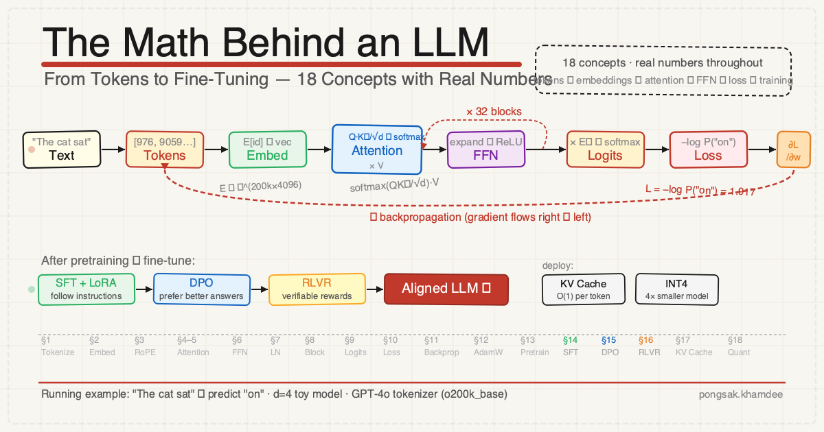
Most LLM explainers either skip the math entirely or dump you into a research paper. This one is neither. We'll walk every equation with real numbers, using the same three-token sentence — "The cat sat" — all the way from raw text to gradient updates.
By the end, you'll be able to trace any weight in any layer and know exactly what changed it, why, and by how much.
This post has a companion: Building an LLM from Scratch in PyTorch implements everything here as working, tested code — 8 phases from a bare transformer to RLHF. This post shows what the machine computes; that one ships it. Read them in either order.
What We're Building Through
Here's the map. Every section uses concrete numbers — no "let x be some vector." Everything is computed.
| Stage | Sections | What you get |
|---|---|---|
| Inference | 1–9 | Forward pass: text in, next token out |
| Learning | 10–12 | Backward pass: loss in, weight update out |
| Pretraining | 13 | The big-scale version of sections 10–12 |
| Fine-tuning | 14–16 | SFT, DPO, RLVR — how raw models become assistants |
| Deployment | 17–18 | KV cache, quantization |
Running setup throughout: sentence "The cat sat", predicting "on". Real token IDs from GPT-4o's o200k_base tokenizer. Embedding dimension d = 4 (real models use 4096+). Vocabulary V = 200,019 tokens.
Prerequisites: multiplication, addition, and patience. Every symbol is decoded in the next section, and every equation is computed with actual numbers — if you can do a dot product, you can follow the whole post.
How to Read the Math
Every symbol used in this article, in one place. Come back here whenever something looks unfamiliar.
Letters and Variables
| Symbol | Read as | Meaning |
|---|---|---|
x | "x" | a single token's embedding vector, e.g. [0.565, 0.540, 0.533, 0.464] |
X | "X" (capital) | the full input matrix — all tokens stacked as rows, shape T×d |
T | "T" | number of tokens in the sequence (e.g. T=3 for "The cat sat") |
d | "d" | embedding dimension — the length of each token vector (4 in toy, 4096 in real) |
V | "V" | vocabulary size — total number of possible tokens (200,019 for GPT-4o) |
L | "L" (loss) | the loss value — a single number measuring how wrong the prediction is |
L | "L" (layers) | number of transformer blocks stacked (32 for Llama 3 8B) |
H | "H" | number of attention heads |
h | "h" | hidden dimension inside FFN (larger than d, e.g. 14,336) |
r | "r" | rank in LoRA — how many dimensions the low-rank matrices use |
m | "m" | position index of a token (position 1, 2, 3…) |
i | "i" | pair index in RoPE (i=0 → first pair of dims, i=1 → second pair…) |
t | "t" | time step in AdamW — which gradient update step we are on |
g | "g" | gradient — the nudge direction computed by backprop |
w | "w" | a single weight value inside a matrix |
θ | "theta" | either (1) all model parameters collectively, or (2) the base rotation angle in RoPE |
α | "alpha" | learning rate — how big each weight update step is (e.g. 2e-4) |
β₁, β₂ | "beta one, beta two" | AdamW momentum decay rates (0.9 and 0.999) |
λ | "lambda" | weight decay coefficient in AdamW (0.01) |
ε | "epsilon" | tiny number added to prevent division by zero (1e-8 or 1e-5) |
γ, β | "gamma, beta" | learned scale and shift in LayerNorm |
μ | "mu" | mean (average) of a vector |
σ | "sigma" | (1) standard deviation, or (2) sigmoid activation function — context tells you which |
π_θ | "pi theta" | the model's probability distribution over outputs |
π_ref | "pi ref" | the frozen reference model used in DPO |
Weight Matrices
| Symbol | Read as | Meaning |
|---|---|---|
E | "E" | embedding matrix — maps token IDs to vectors, shape V×d |
Eᵀ | "E transpose" | E flipped — rows become columns. Used at output to convert vectors back to vocab scores |
W_Q | "W Q" | query weight matrix — projects x into "what am I looking for?" space |
W_K | "W K" | key weight matrix — projects x into "what do I contain?" space |
W_V | "W V" | value weight matrix — projects x into "what will I pass along?" space |
W_O | "W O" | output weight matrix — projects concatenated heads back to model dimension |
W_gate | "W gate" | gating weight matrix in SwiGLU FFN — controls which neurons fire |
W₁ | "W one" | first FFN weight matrix — expands d → h |
W₂ | "W two" | second FFN weight matrix — contracts h → d |
I | "identity" | identity matrix — multiplying by I changes nothing (like multiplying by 1) |
Math Symbols
| Symbol | Read as | Meaning | Example |
|---|---|---|---|
∈ | "is in" / "belongs to" | "has the type" or "is a member of" | W_Q ∈ ℝ^(d×d) = "W_Q is a real-valued d×d matrix" |
ℝ | "real numbers" | the set of all ordinary decimal numbers (floats) | ℝ^(3×4) = a 3-row, 4-column grid of floats |
^(m×n) | "shape m by n" | a matrix with m rows and n columns | ℝ^(200019×4096) = 200,019 rows, 4,096 cols |
· | "dot" | (1) dot product between two vectors, or (2) matrix multiply | Q · Kᵀ = matrix multiply Q by K-transposed |
× | "times" | ordinary multiplication, or matrix dimensions | 3×4 = 3 rows by 4 columns |
⊙ | "hadamard" / "element-wise times" | multiply two vectors position by position | [1,2] ⊙ [3,4] = [3,8] |
ᵀ | "transpose" | flip a matrix — rows become columns | Kᵀ = K with rows and columns swapped |
√ | "square root" | √4 = 2 | |
∂L/∂w | "partial L over partial w" | gradient — how much the loss L changes if weight w moves slightly | ∂L/∂w = -0.853 means increasing w decreases loss |
Σ | "sum" | add everything up | Σᵢ xᵢ = x₁ + x₂ + x₃ + … |
−∞ | "negative infinity" | a value so negative that e^(−∞) = 0 — used to mask future tokens in softmax | |
log | "log" | natural logarithm (base e) | log(1.0) = 0, log(0.147) = −1.917 |
e^x | "e to the x" | exponential function — always positive, grows fast | e^0 = 1, e^1 = 2.718 |
max(0, x) | "max of zero and x" | ReLU — returns x if positive, zero if negative | max(0, -0.3) = 0, max(0, 0.8) = 0.8 |
≈ | "approximately equal" | close but not exact | e^0.43 ≈ 1.537 |
≪ | "much less than" | far smaller | r ≪ d means rank 16 is far smaller than dim 4096 |
1[condition] | "indicator of condition" | equals 1 if condition is true, 0 if false | 1[token = "on"] = 1 only for "on", 0 for everything else |
How to Read a Full Equation Out Loud
"W_Q is a matrix of real numbers with shape d-by-d."
"The attention output equals: softmax of Q times K-transpose, divided by the square root of d_k, then multiplied by V."
"The gradient of the loss with respect to logit z-i equals: the model's predicted probability for token i, minus one if token i is the correct token, otherwise minus zero."
"Update theta by subtracting: alpha times m-hat over root-v-hat-plus-epsilon (the gradient step), then also subtracting alpha times lambda times theta (the weight decay)."
1. Tokenization
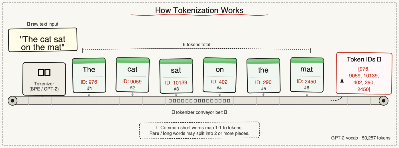
The model never sees letters. It sees integers. A tokenizer maps text to IDs using a pre-built vocabulary.
Run this yourself with GPT-4o's tokenizer:
import tiktoken
enc = tiktoken.get_encoding("o200k_base")

enc.encode("The cat sat on the mat")
# [976, 9059, 10139, 402, 290, 2450]

# Each token decoded back to text:
[enc.decode([t]) for t in [976, 9059, 10139, 402, 290, 2450]]
# ['The', ' cat', ' sat', ' on', ' the', ' mat']
Those six integers are all the model receives. The vocabulary has 200,019 possible IDs — each one a pre-built subword unit:
Token ID  →  Text
─────────────────────────
     976  →  "The"        (common word → single token)
    9059  →  " cat"       (space included inside the token)
   10139  →  " sat"
     402  →  " on"
     290  →  " the"       (lowercase "the" is a different ID from "The"=976)
    2450  →  " mat"
Real tokenizers (GPT-4o uses o200k_base) split on subwords using Byte-Pair Encoding (BPE):
- Start with individual bytes as tokens.
- Count the most frequent adjacent pair across the corpus.
- Merge it into a new single token.
- Repeat until vocabulary size is reached.
"tokenization" → ["token", "ization"] — two tokens because "ization" is a common suffix. This is why you pay per token, not per word. "antidisestablishmentarianism" is one word but 6 tokens.
For our worked example: [976, 9059, 10139] — the IDs for "The cat sat". These three integers are all that enters the model.
2. Vector Embeddings
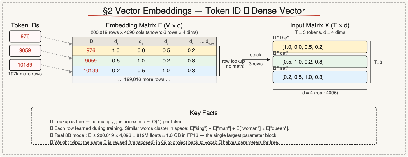
Token ID 9059 means nothing on its own — it's just a row index. An embedding matrix E ∈ ℝ^(V×d) maps each ID to a dense vector of dimension d.
Reading that notation: E is the matrix name, ∈ means "is a matrix of", ℝ means real numbers (floats), V×d is the shape — V rows by d columns. One row per vocabulary token.
In a real model: E is 200,019 × 4096 — about 800 million numbers for the embedding layer alone. We're showing 6 rows out of 200,019, shrunk to d=4 for readability:
E  (200,019 × 4096 in reality; shown as 6 rows × 4 dims)
         d₁    d₂    d₃    d₄
   976 | 1.0   0.0   0.5   0.2 |  ← "The"
  9059 | 0.5   1.0   0.2   0.8 |  ← " cat"
 10139 | 0.2   0.5   1.0   0.3 |  ← " sat"
   402 | 0.7   0.1   0.4   0.6 |  ← " on"
   290 | 0.9   0.1   0.5   0.2 |  ← " the"   (note: ID 290 ≠ ID 976)
  2450 | 0.4   0.9   0.1   0.7 |  ← " mat"
Embedding lookup is just row indexing — no computation at all. Token ID 9059 → row 9059 of E:
E[976]   = [1.0, 0.0, 0.5, 0.2]   ← "The"
E[9059]  = [0.5, 1.0, 0.2, 0.8]   ← " cat"
E[10139] = [0.2, 0.5, 1.0, 0.3]   ← " sat"
Stack those three rows into the input matrix X ∈ ℝ^(T×d) where T=3:
X =
| 1.0   0.0   0.5   0.2 |  ← row 976   "The"    (position 1)
| 0.5   1.0   0.2   0.8 |  ← row 9059  " cat"   (position 2)
| 0.2   0.5   1.0   0.3 |  ← row 10139 " sat"   (position 3)
These 12 numbers (3 tokens × 4 dims) are the model's entire input. They were learned during training — not hand-designed. A real 4096-dim embedding packs 4096 floats per token, encoding everything the model knows about that subword's meaning and usage across the training corpus.
3. Positional Encoding: RoPE
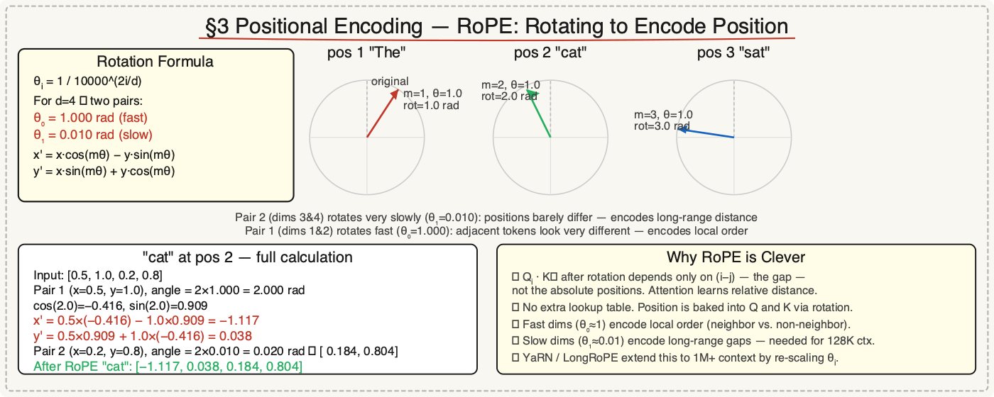
Plain attention has no concept of word order — X has no idea that "cat" comes before "sat." RoPE (Rotary Position Embedding) encodes position by rotating each token's Query and Key vectors.
The idea: take a token's dimensions in pairs (x₂ᵢ₋₁, x₂ᵢ) and rotate each pair by angle mθᵢ, where m is the token's position.
Reading the pair notation: for
x = [x₁, x₂, x₃, x₄](d=4), the pairs are:
i=0→ pair(x₁, x₂)— dims 1 & 2i=1→ pair(x₃, x₄)— dims 3 & 4
Each pair gets its own base angle:
For d=4 we have two pairs, so two base angles (rad - radian):
Rotation formula for a pair (x, y) by angle θ:
"cat" is at position m=2, embedding [0.5, 1.0, 0.2, 0.8]:
Pair 1 (0.5, 1.0), angle 2 × 1.000 = 2.000 rad:
cos(2.0) = −0.416,  sin(2.0) = 0.909
x' = 0.5×(−0.416) − 1.0×0.909 = −0.208 − 0.909 = −1.117
y' = 0.5×0.909  + 1.0×(−0.416) = 0.454 − 0.416 =  0.038
Pair 2 (0.2, 0.8), angle 2 × 0.010 = 0.020 rad:
cos(0.02) ≈ 0.9998,  sin(0.02) ≈ 0.020
x' = 0.2×0.9998 − 0.8×0.020 = 0.200 − 0.016 =  0.184
y' = 0.2×0.020  + 0.8×0.9998 = 0.004 + 0.800 =  0.804
After RoPE, "cat" at position 2: [−1.117, 0.038, 0.184, 0.804]
One honesty note before moving on: in a real model, RoPE rotates the Q and K vectors (after the
W_Q/W_Kprojections in Section 4), not the raw embedding. We rotated the embedding here to show the arithmetic in one place — and to keep Section 4's numbers easy to follow, the attention walkthrough below uses the unrotatedX. The rotation math is identical wherever you apply it. (The build post implements RoPE the production way — applied to Q and K, in ~15 lines of PyTorch.)
Why this is clever: when you compute the dot product (attention score-how relevant "cat" is to "sat") Qᵢ · Kⱼ after rotation, the result depends only on the relative distance i−j (i − j is the gap between any two tokens. Example: "sat" (position 3) looking at "The" (position 1) → 3 − 1 = 2 steps apart), not the absolute positions. That's what gives attention its sense of "how far apart are these two tokens" without needing a position lookup table. It also scales to longer contexts with techniques like YaRN.
4. Attention: Q, K, and V
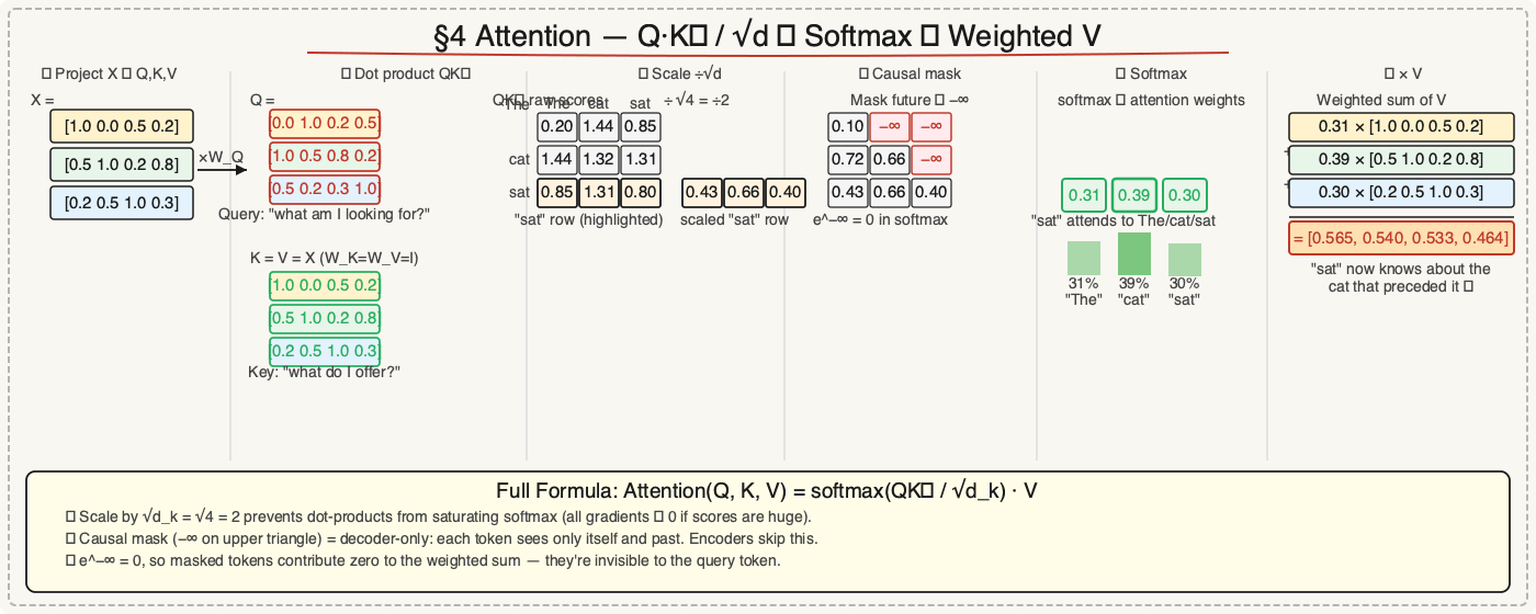
This is the engine. Attention lets each token gather information from every other token — weighted by relevance.
Step 1 — Project to Q, K, V
Three learned weight matrices W_Q, W_K, W_V ∈ ℝ^(d×d) project X into Queries, Keys, and Values:
| Matrix | Projects each token into | Intuition |
|---|---|---|
W_Q | a Query | what the token is looking for — "I'm 'sat', what do I need to know?" |
W_K | a Key | what the token contains — "I'm 'cat', here's what I'm about" |
W_V | a Value | what the token passes along if attended to — "if you pick me, here's what you get" |
So W_Q ∈ ℝ^(d×d) reads: "W_Q is a matrix of real numbers with shape d×d" (the symbol tables above decode every piece).
For our example, use these weight matrices:
W_K = W_V = I means K = V = X. W_Q shuffles the columns of X, so Q ≠ X.
Compute Q = X · W_Q:
Row 1 ("The"): [1.0, 0.0, 0.5, 0.2] · W_Q

  Multiply against each column, here is example:
  q₁[1] = x · c₁ = 1.0×0 + 0.0×1 + 0.5×0 + 0.2×0 = 0.0
  q₁[2] = x · c₂ = 1.0×1 + 0.0×0 + 0.5×0 + 0.2×0 = 1.0
  q₁[3] = x · c₃ = 1.0×0 + 0.0×0 + 0.5×0 + 0.2×1 = 0.2
  q₁[4] = x · c₄ = 1.0×0 + 0.0×0 + 0.5×1 + 0.2×0 = 0.5

  q₁ = [0.0, 1.0, 0.2, 0.5]

Row 2 ("cat"): [0.5, 1.0, 0.2, 0.8] · W_Q
  q₂ = [1.0, 0.5, 0.8, 0.2]

Row 3 ("sat"): [0.2, 0.5, 1.0, 0.3] · W_Q
  q₃ = [0.5, 0.2, 0.3, 1.0]
Q =                     K = X =                 V = X =
| 0.0  1.0  0.2  0.5 |  | 1.0  0.0  0.5  0.2 |  | 1.0  0.0  0.5  0.2 | ← "The"
| 1.0  0.5  0.8  0.2 |  | 0.5  1.0  0.2  0.8 |  | 0.5  1.0  0.2  0.8 | ← " cat"
| 0.5  0.2  0.3  1.0 |  | 0.2  0.5  1.0  0.3 |  | 0.2  0.5  1.0  0.3 | ← " sat"
Step 2 — Compute Attention Scores
The full attention formula: Attention(Q, K, V) = softmax(QKᵀ / √d_k) · V
First, QKᵀ (3×3). Each cell is a dot product qᵢ · kⱼ:
Dot product = multiply each pair of matching numbers, then add them all up.
Score("sat","The") = q₃ · k₁ = 0.5×1.0 + 0.2×0.0 + 0.3×0.5 + 1.0×0.2
                              = 0.50 + 0.00 + 0.15 + 0.20 = 0.85

Score("sat","cat") = q₃ · k₂ = 0.5×0.5 + 0.2×1.0 + 0.3×0.2 + 1.0×0.8
                              = 0.25 + 0.20 + 0.06 + 0.80 = 1.31

Score("sat","sat") = q₃ · k₃ = 0.5×0.2 + 0.2×0.5 + 0.3×1.0 + 1.0×0.3
                              = 0.10 + 0.10 + 0.30 + 0.30 = 0.80
Full QKᵀ matrix:
Step 3 — Scale
Divide by √d_k = √4 = 2 to stop the dot products from getting so large that softmax saturates:
QKᵀ / √d_k =
              "The"   "cat"   "sat"
"The"  |  0.10    0.72    0.43  |
"cat"  |  0.72    0.66    0.66  |
"sat"  |  0.43    0.66    0.40  |
Step 4 — Causal Mask
This is a decoder (language model), so each token can only attend to past tokens and itself — not the future. Mask future positions with −∞:
Step 5 — Softmax
softmax(xᵢ) = e^xᵢ / Σⱼ e^xⱼ (e^(−∞) = 0, so masked positions vanish)
For "sat" → scores [0.43, 0.66, 0.40]:
e^0.43 = 1.537
e^0.66 = 1.935
e^0.40 = 1.492
sum    = 4.964

attention weights = [1.537/4.964, 1.935/4.964, 1.492/4.964]
                  = [0.31,        0.39,         0.30       ]
                      ↑             ↑             ↑
                    "The"         "cat"         "sat"
"sat" cares most about "cat" (39%), then "The" (31%), then itself (30%).
Step 6 — Weighted Sum of Values
Output("sat") = 0.31 × V_The + 0.39 × V_cat + 0.30 × V_sat

= 0.31 × [1.0, 0.0, 0.5, 0.2]
+ 0.39 × [0.5, 1.0, 0.2, 0.8]
+ 0.30 × [0.2, 0.5, 1.0, 0.3]

= [0.310, 0.000, 0.155, 0.062]
+ [0.195, 0.390, 0.078, 0.312]
+ [0.060, 0.150, 0.300, 0.090]

= [0.565, 0.540, 0.533, 0.464]   ← "sat" after attending to context
The number [0.565, 0.540, 0.533, 0.464] is a blend of all three tokens' values, weighted by how relevant each one was to "sat's" query. "sat" now "knows" about the cat that preceded it.
Everything in this section is ~30 lines of PyTorch — the MultiHeadAttention class in Phase 1 of the build post is this exact math, vectorised.
5. Multi-Head Attention
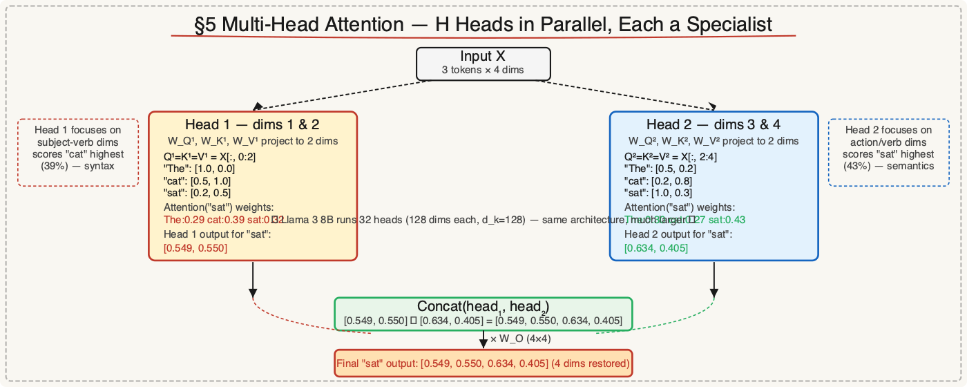
One attention head tracks one type of relationship. Multi-head attention runs H heads in parallel, each learning a different relationship type (subject-verb, pronoun-referent, syntactic distance...).
For d=4, H=2: each head gets d_k = d/H = 2 dimensions. Each head has its own slim projection matrices of shape 4×2 instead of 4×4.
Head 1 — focuses on dims 1 & 2
W_Q¹ = W_K¹ = W_V¹ =        W_Q² = W_K² = W_V² =
| 1  0 |                      | 0  0 |
| 0  1 |                      | 0  0 |
| 0  0 |                      | 1  0 |
| 0  0 |                      | 0  1 |
Q¹ = K¹ = V¹ = X · W_Q¹ — slices the first two columns of X:
Attention scores for "sat" (Q¹₃ · K¹ᵀ), scaled by √d_k = √2 = 1.414:
[0.2, 0.5] · [1.0, 0.0] = 0.20  →  0.20/1.414 = 0.14
[0.2, 0.5] · [0.5, 1.0] = 0.60  →  0.60/1.414 = 0.42
[0.2, 0.5] · [0.2, 0.5] = 0.29  →  0.29/1.414 = 0.21
Softmax [0.14, 0.42, 0.21]:
Head 1 output for "sat":
0.29×[1.0, 0.0] + 0.39×[0.5, 1.0] + 0.32×[0.2, 0.5]
= [0.290, 0.000] + [0.195, 0.390] + [0.064, 0.160]
= [0.549, 0.550]
Head 2 — focuses on dims 3 & 4
Q² = K² = V² = X · W_Q² — slices the last two columns of X:
Attention scores for "sat", scaled by √2:
[1.0, 0.3] · [0.5, 0.2] = 0.56  →  0.56/1.414 = 0.40
[1.0, 0.3] · [0.2, 0.8] = 0.44  →  0.44/1.414 = 0.31
[1.0, 0.3] · [1.0, 0.3] = 1.09  →  1.09/1.414 = 0.77
Softmax [0.40, 0.31, 0.77]:
Head 2 output for "sat":
0.30×[0.5, 0.2] + 0.27×[0.2, 0.8] + 0.43×[1.0, 0.3]
= [0.150, 0.060] + [0.054, 0.216] + [0.430, 0.129]
= [0.634, 0.405]
Concatenate → Project
Head 1 output: [0.549, 0.550]             (2 dims)
Head 2 output: [0.634, 0.405]             (2 dims)
                    ↓ concat
               [0.549, 0.550, 0.634, 0.405]   (back to 4 dims)
                    ↓ × W_O (4×4, identity here)
Final output:  [0.549, 0.550, 0.634, 0.405]
What the two heads saw differently:
- Head 1 scored
"cat"highest (0.39) — tracking subject-verb relationships in dims 1–2 - Head 2 scored
"sat"highest (0.43) — tracking action/verb features in dims 3–4
The concatenated vector carries both views in one pass. A real model like Llama 3 8B runs 32 heads simultaneously, each a 128-dim specialist — none of them assigned their job by hand; they specialize during training.
One modern wrinkle: those 32 query heads share only 8 key/value heads. That's Grouped-Query Attention (GQA) — every group of 4 query heads reads the same K and V. It cuts the KV cache (Section 17) to a quarter with negligible quality loss, which is why virtually every 2026 model (Llama, Qwen, Mistral, Gemma) uses it.
6. Feed-Forward Network
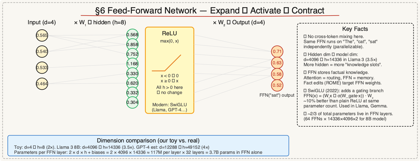
After attention, each token passes through an FFN independently — no token-to-token mixing here. This is where factual knowledge lives.
The formula (using SwiGLU, the modern standard in Llama, Qwen, and Mistral):
For the worked example we'll use the simpler classic version: FFN(x) = ReLU(xW₁ + b₁)W₂ + b₂. Same shape — expand, apply a nonlinearity, contract — SwiGLU just adds a learned gate that decides how much of each hidden neuron passes through.
| Symbol | Name | Meaning |
|---|---|---|
x | input | token vector coming in, shape (1 × d), e.g. [0.565, 0.540, 0.533, 0.464] |
W₁ | weight matrix 1 | learned matrix, shape (d × h) — expands from d=4 → h=8 |
xW₁ | matrix multiply | project x into larger hidden space, result shape (1 × h) |
b₁ | bias 1 | learned vector, shape (1 × h) — shifts each neuron up or down |
xW₁ + b₁ | pre-activation | raw hidden values before activation function |
ReLU(...) | activation | max(0, x) — kills negative values, keeps positive ones unchanged |
W₂ | weight matrix 2 | learned matrix, shape (h × d) — contracts back from h=8 → d=4 |
b₂ | bias 2 | learned vector, shape (1 × d) — final shift on the output |
Setup: d=4, hidden size h=8. Real models expand 3–4×: Llama 3 8B uses h=14,336 ≈ 3.5 × 4096.
Input: x = [0.565, 0.540, 0.533, 0.464] (the "sat" output from attention)
W₁ ∈ ℝ^(4×8) (each column is one hidden neuron's weights):
W₁ =
|  1.0   0.5  -0.5   1.0  -1.0   0.5   1.0  -0.5 |
|  0.5   1.0   0.5   0.5  -0.5  -0.5   0.0   0.5 |
| -0.5   0.5   1.0   0.5   0.5   0.5  -1.0  -0.5 |
|  0.0  -0.5   0.5  -0.5   0.5   1.0   0.5   1.0 |
Compute h = x · W₁ + b₁ (with b₁ = 0 for simplicity). Each hₙ = x dotted with column n of W₁:
h₁ = 0.565×1.0  + 0.540×0.5  + 0.533×(−0.5) + 0.464×0.0
   = 0.565 + 0.270 − 0.267 + 0.000 = 0.568

h₂ = 0.565×0.5  + 0.540×1.0  + 0.533×0.5   + 0.464×(−0.5)
   = 0.283 + 0.540 + 0.267 − 0.232 = 0.858

h₃ = 0.565×(−0.5) + 0.540×0.5  + 0.533×1.0  + 0.464×0.5
   = −0.283 + 0.270 + 0.533 + 0.232 = 0.752

h₄ = 0.565×1.0  + 0.540×0.5  + 0.533×0.5   + 0.464×(−0.5)
   = 0.565 + 0.270 + 0.267 − 0.232 = 0.870

h₅ = 0.565×(−1.0) + 0.540×(−0.5) + 0.533×0.5  + 0.464×0.5
   = −0.565 − 0.270 + 0.267 + 0.232 = −0.336   ← negative

h₆ = 0.565×0.5  + 0.540×(−0.5) + 0.533×0.5   + 0.464×1.0
   = 0.283 − 0.270 + 0.267 + 0.464 = 0.744

h₇ = 0.565×1.0  + 0.540×0.0   + 0.533×(−1.0) + 0.464×0.5
   = 0.565 + 0.000 − 0.533 + 0.232 = 0.264

h₈ = 0.565×(−0.5) + 0.540×0.5  + 0.533×(−0.5) + 0.464×1.0
   = −0.283 + 0.270 − 0.267 + 0.464 = 0.184
Full hidden vector before ReLU:
Apply ReLU: max(0, x) — h₅ is negative, so it gets zeroed out:
ReLU(h):
  h₁ = max(0,  0.568) =  0.568
  h₂ = max(0,  0.858) =  0.858
  h₃ = max(0,  0.752) =  0.752
  h₄ = max(0,  0.870) =  0.870
  h₅ = max(0, −0.336) =  0.000  ← killed by ReLU
  h₆ = max(0,  0.744) =  0.744
  h₇ = max(0,  0.264) =  0.264
  h₈ = max(0,  0.184) =  0.184
h₅ was detecting a pattern that doesn't apply to "sat" — ReLU silences it. After ReLU: h = [0.568, 0.858, 0.752, 0.870, 0.000, 0.744, 0.264, 0.184]
Then W₂ ∈ ℝ^(8×4) projects back to d=4. Each ROW of W₂ = how one hidden neuron spreads its value across the 4 output dims:
W₂ =            out₁  out₂  out₃  out₄
h₁ row →  |  0.5   0.2   0.1   0.1 |
h₂ row →  |  0.1   0.3   0.2   0.1 |
h₃ row →  |  0.2   0.1   0.3   0.1 |
h₄ row →  |  0.1   0.2   0.1   0.3 |
h₅ row →  |  0.0   0.0   0.0   0.0 |  ← h₅=0 so this whole row contributes nothing
h₆ row →  |  0.1   0.1   0.1   0.2 |
h₇ row →  |  0.2   0.1   0.1   0.1 |
h₈ row →  |  0.1   0.1   0.2   0.1 |
Compute each output dimension by summing hᵢ × W₂[i, col] down the column:
out₁ = 0.568×0.5 + 0.858×0.1 + 0.752×0.2 + 0.870×0.1 + 0×0.0 + 0.744×0.1 + 0.264×0.2 + 0.184×0.1
     = 0.284     + 0.086     + 0.150     + 0.087     + 0.000 + 0.074     + 0.053     + 0.018
     = 0.753

out₂ = 0.568×0.2 + 0.858×0.3 + 0.752×0.1 + 0.870×0.2 + 0×0.0 + 0.744×0.1 + 0.264×0.1 + 0.184×0.1
     = 0.114     + 0.257     + 0.075     + 0.174     + 0.000 + 0.074     + 0.026     + 0.018
     = 0.739

out₃ = 0.568×0.1 + 0.858×0.2 + 0.752×0.3 + 0.870×0.1 + 0×0.0 + 0.744×0.1 + 0.264×0.1 + 0.184×0.2
     = 0.057     + 0.172     + 0.226     + 0.087     + 0.000 + 0.074     + 0.026     + 0.037
     = 0.679

out₄ = 0.568×0.1 + 0.858×0.1 + 0.752×0.1 + 0.870×0.3 + 0×0.0 + 0.744×0.2 + 0.264×0.1 + 0.184×0.1
     = 0.057     + 0.086     + 0.075     + 0.261     + 0.000 + 0.149     + 0.026     + 0.018
     = 0.672
Notice h₅ contributes zero to every output dim — ReLU already zeroed it, so its entire W₂ row is irrelevant. That neuron is completely silent for this token.
The FFN runs identically on every token position. "The", "cat", and "sat" each get their own FFN pass — no cross-token communication at this stage.
7. Layer Normalization
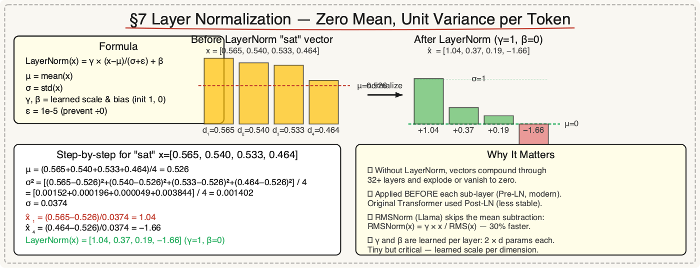
Raw vectors tend to drift in scale as they pass through layers. Layer norm re-centers and rescales each token's vector before attention and FFN.
Formula for a vector x ∈ ℝ^d:
μ= mean ofxσ= standard deviation ofxγ, β= learned scale and bias (initialized to 1 and 0)ε = 1e-5(numerical stability)
For "sat" after attention: x = [0.565, 0.540, 0.533, 0.464]
μ = (0.565 + 0.540 + 0.533 + 0.464) / 4 = 0.526

σ² = [(0.565−0.526)² + (0.540−0.526)² + (0.533−0.526)² + (0.464−0.526)²] / 4
   = [0.00152 + 0.000196 + 0.000049 + 0.003844] / 4
   = 0.001402
σ  = 0.0374

Normalized (each of the 4 dimensions of "sat"'s vector):
  (0.565 − 0.526) / 0.0374 = 1.04
  (0.540 − 0.526) / 0.0374 = 0.37
  (0.533 − 0.526) / 0.0374 = 0.19
  (0.464 − 0.526) / 0.0374 = −1.66
With γ=1, β=0: LayerNorm(x) = [1.04, 0.37, 0.19, −1.66]
The values now have zero mean and unit variance. Without this step, values compound multiplicatively through dozens of layers and blow up or collapse to zero.
2026 reality check: Llama, Qwen, and Mistral actually use RMSNorm, a cheaper cousin that skips the mean subtraction entirely:
Same job — keep scales stable — with one less statistic to compute per token per layer. If you read a modern model's source, this is the norm you'll find.
8. Transformer Block
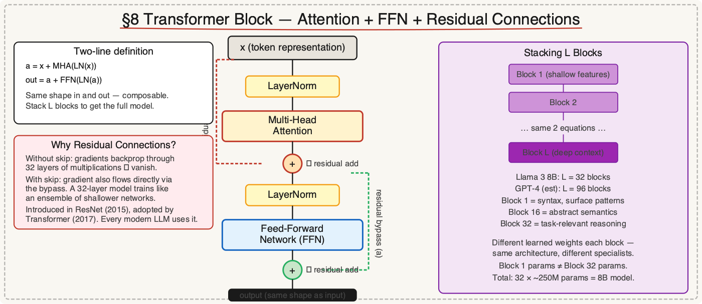
Sections 4–7 don't run once — they form a block, and the full model stacks L identical blocks.
One block in full:
a  = x + MultiHeadAttention(LayerNorm(x))    ← residual + attention
out = a + FFN(LayerNorm(a))                  ← residual + FFN
The +x parts are residual connections — a bypass lane from input to output that lets gradients flow backward without vanishing. Without them, a 32-layer model simply won't train.
Llama 3 8B stacks 32 of these blocks. The same block architecture repeats — what differs are the learned weights inside each block. Token representations enter block 1 shallow and context-free; they exit block 32 rich with long-range context and factual associations.
9. Output Projection and Logits
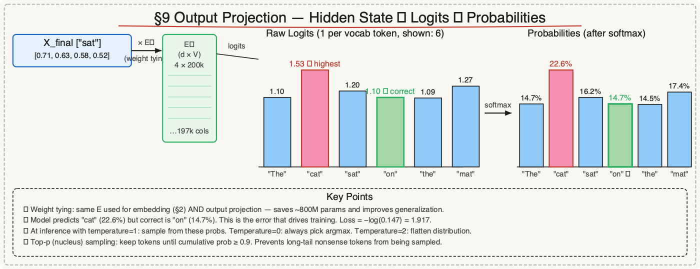
After the last block, we have a final hidden state for each position. To predict the next token, we need a score for every vocabulary item.
The language model head projects back to vocabulary size:
We reuse the embedding matrix E transposed (weight tying — a common trick that halves parameters). Each token in the final hidden state gets a dot product with every vocabulary embedding.
For "sat" at position 3, X_final[3] = [0.71, 0.63, 0.58, 0.52]:
logit("The") = [0.71,0.63,0.58,0.52] · [1.0, 0.0, 0.5, 0.2] = 0.71+0+0.29+0.10 = 1.10
logit("cat") = [0.71,0.63,0.58,0.52] · [0.5, 1.0, 0.2, 0.8] = 0.36+0.63+0.12+0.42 = 1.53
logit("sat") = [0.71,0.63,0.58,0.52] · [0.2, 0.5, 1.0, 0.3] = 0.14+0.32+0.58+0.16 = 1.20
logit("on")  = [0.71,0.63,0.58,0.52] · [0.7, 0.1, 0.4, 0.6] = 0.50+0.06+0.23+0.31 = 1.10
logit("the") = [0.71,0.63,0.58,0.52] · [0.9, 0.1, 0.5, 0.2] = 0.64+0.06+0.29+0.10 = 1.09
logit("mat") = [0.71,0.63,0.58,0.52] · [0.4, 0.9, 0.1, 0.7] = 0.28+0.57+0.06+0.36 = 1.27
Apply softmax to turn logits into probabilities:
logits: [1.10, 1.53, 1.20, 1.10, 1.09, 1.27]

e^1.10 = 3.00,  e^1.53 = 4.62,  e^1.20 = 3.32
e^1.10 = 3.00,  e^1.09 = 2.97,  e^1.27 = 3.56
sum = 20.47

P("The") = 3.00/20.47 = 14.7%
P("cat") = 4.62/20.47 = 22.6%   ← highest but wrong (correct is "on")
P("sat") = 3.32/20.47 = 16.2%
P("on")  = 3.00/20.47 = 14.7%
P("the") = 2.97/20.47 = 14.5%
P("mat") = 3.56/20.47 = 17.4%
The model predicts "cat" (22.6%) but the correct next token is "on" (14.7%). That's the error we'll fix in the next three sections.
(We're showing 6 vocabulary entries for readability. A real model computes this softmax over all 200,019 logits, every single decode step — the other 200,013 tokens each get a sliver of the remaining probability.)
10. Cross-Entropy Loss
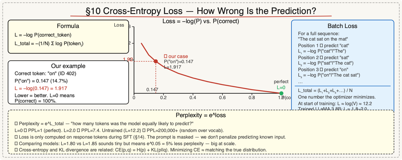
Loss measures how wrong the prediction is. We want the probability of the correct token to be as high as possible.
Cross-entropy loss for a single prediction:
Correct token is "on" (ID 4), P("on") = 0.147:
The lower the loss, the better. L=0 means P(correct) = 1.0 — a perfect prediction. L=1.917 means the model is quite uncertain.
Over a full training batch, we average the loss across all positions and all sequences:
This is the single number the entire learning machinery minimizes.
11. Backpropagation
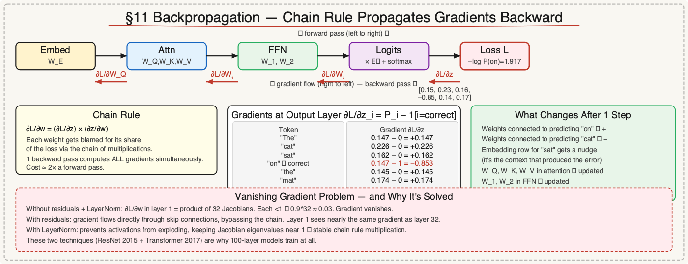
The loss is a number. But there are billions of weights. Backpropagation computes how much each weight contributed to the loss — the gradient — using the chain rule from calculus.
The chain rule: if L depends on z, which depends on w:
Chain this backward through every layer: output → FFN → attention → embeddings.
Concrete example — gradient at the output layer:
At the output softmax, the gradient of loss w.r.t. logit zᵢ is:
For our case (correct = "on", ID 4):
∂L/∂z("The")  = 0.147 − 0  =  0.147
∂L/∂z("cat")  = 0.226 − 0  =  0.226
∂L/∂z("sat")  = 0.162 − 0  =  0.162
∂L/∂z("on")   = 0.147 − 1  = −0.853   ← strong negative gradient: push "on" higher
∂L/∂z("the")  = 0.145 − 0  =  0.145
∂L/∂z("mat")  = 0.174 − 0  =  0.174
The −0.853 on "on" tells the model: the weights connected to predicting "on" need to grow. Every other token's gradient is positive: those weights need to shrink slightly.
This gradient vector flows backward through Eᵀ, then through the last transformer block's FFN, then through the FFN's weight matrices W₂ and W₁, then through the attention layers, and finally into the embedding matrix E. Each weight gets a number: which direction to move and by how much.
One backward pass computes gradients for all billions of weights simultaneously. It's computationally about 2× the cost of a forward pass.
12. AdamW Optimizer
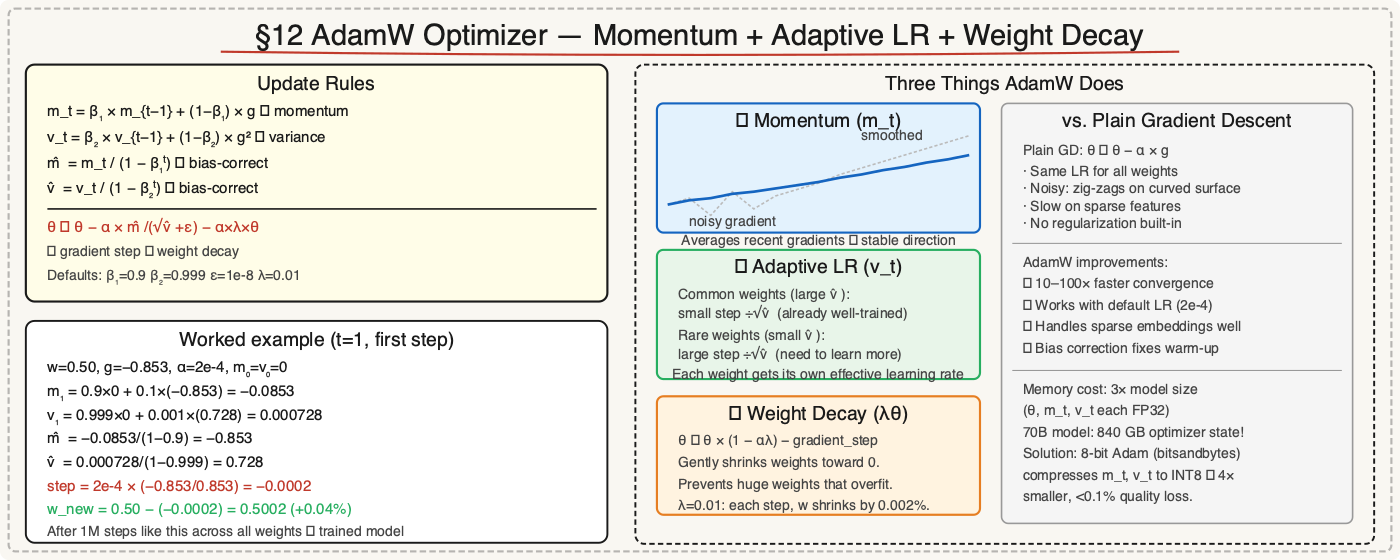
Backprop computes gradients g. The optimizer turns gradients into actual weight updates.
AdamW update rule (the standard for LLM training):
m_t = β₁ × m_{t−1} + (1−β₁) × g          ← first moment (momentum)
v_t = β₂ × v_{t−1} + (1−β₂) × g²         ← second moment (variance)

m̂ = m_t / (1 − β₁ᵗ)                       ← bias correction
v̂ = v_t / (1 − β₂ᵗ)                       ← bias correction

θ ← θ − α × m̂ / (√v̂ + ε)  − α × λ × θ  ← update + weight decay
Default hyperparameters: β₁=0.9, β₂=0.999, ε=1e-8, λ=0.01
Concrete example — updating one weight:
Say weight w = 0.50, gradient g = −0.853 (the "on" logit gradient), learning rate α = 2e-4, first step (t=1):
m₁ = 0.9×0.000 + 0.1×(−0.853) = −0.0853
v₁ = 0.999×0.000 + 0.001×(0.853²) = 0.000728

m̂ = −0.0853 / (1 − 0.9)  = −0.853
v̂ = 0.000728 / (1 − 0.999) = 0.728

update = 2e-4 × (−0.853) / (√0.728 + 1e-8)
       = 2e-4 × (−0.853) / 0.853
       = 2e-4 × (−1.000)
       = −0.0002

weight_decay = 2e-4 × 0.01 × 0.50 = 0.000001

New w = 0.50 − (−0.0002) − 0.000001 = 0.5002
The weight moved from 0.50 to 0.5002 — a tiny step toward predicting "on" more confidently. Repeat across all billions of weights, across trillions of examples. That's training.
Three things AdamW does that plain gradient descent can't: - Momentum (m_t): averages recent gradients so noisy batches don't jerk weights around wildly. - Adaptive scaling (v_t): weights that get large, consistent gradients get smaller steps; rare gradients get larger steps. - Weight decay (λθ): gently shrinks weights toward zero unless gradients justify keeping them large — prevents overfitting.
13. Pretraining
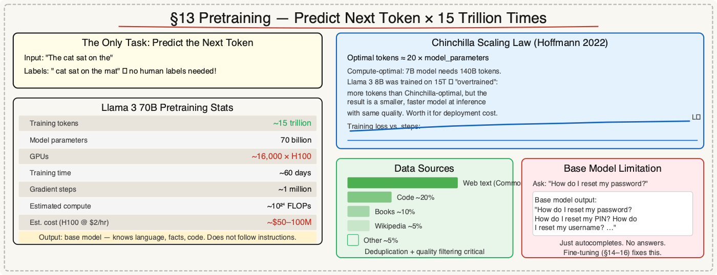
Sections 10–12 run on a single example. Pretraining scales this to ~15 trillion tokens across every text on the internet.
The task is always the same: predict the next token. No human labels required — the next word in the actual text is the label. This is called self-supervised learning.
Scale of a real pretraining run (Llama 3 70B):
| Quantity | Value |
|---|---|
| Training tokens | ~15 trillion |
| Model parameters | 70 billion |
| GPUs | ~16,000 × H100 |
| Training time | ~60 days |
| Gradient steps | ~1 million |
The Chinchilla scaling law (Hoffmann et al. 2022) says the optimal compute split is roughly equal tokens and parameters:
A 7B model trained on ~140B tokens is compute-optimal. Most modern models overtrain relative to this (more tokens than Chinchilla-optimal) to produce smaller inference-time models.
The result of pretraining: a base model — knows language, facts, code. But it just autocompletes text. Ask "How do I reset my password?" and it'll generate more questions, not an answer. That's the next step's job.
14. Fine-Tuning: SFT (Supervised Fine-Tuning)
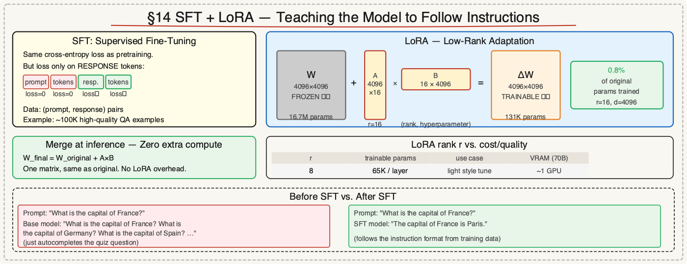
A base model has no "answer a question" behavior. SFT teaches it by training on thousands of high-quality (prompt, response) pairs.
The loss function is identical to pretraining's cross-entropy — but only computed on the response tokens, not the prompt:
We don't want to optimize predicting the prompt — that's fixed. We only penalize wrong response tokens.
Prompt:   "What comes after a cat sat on the ___?"
Response: "mat"
Loss:     −log P("mat" | prompt) = −log P("mat" | "What comes after...")
LoRA (Low-Rank Adaptation) is the dominant SFT method in 2026. Instead of updating all 70B weights (which requires 70B+ of optimizer state), it injects small trainable matrices into each attention layer:
For d=4096, r=16: original matrix has 4096²=16.7M parameters. LoRA adds 2×4096×16=131K — just 0.8% of the original. Train only A and B, freeze everything else.
At inference, merge: W_final = W_original + A×B. Zero extra compute.
Want to run this? Phase 6 of the build post implements the response-masked loss and a working LoRALinear class — including the sanity check that the adapter starts as an exact identity.
15. Fine-Tuning: DPO (Direct Preference Optimization)
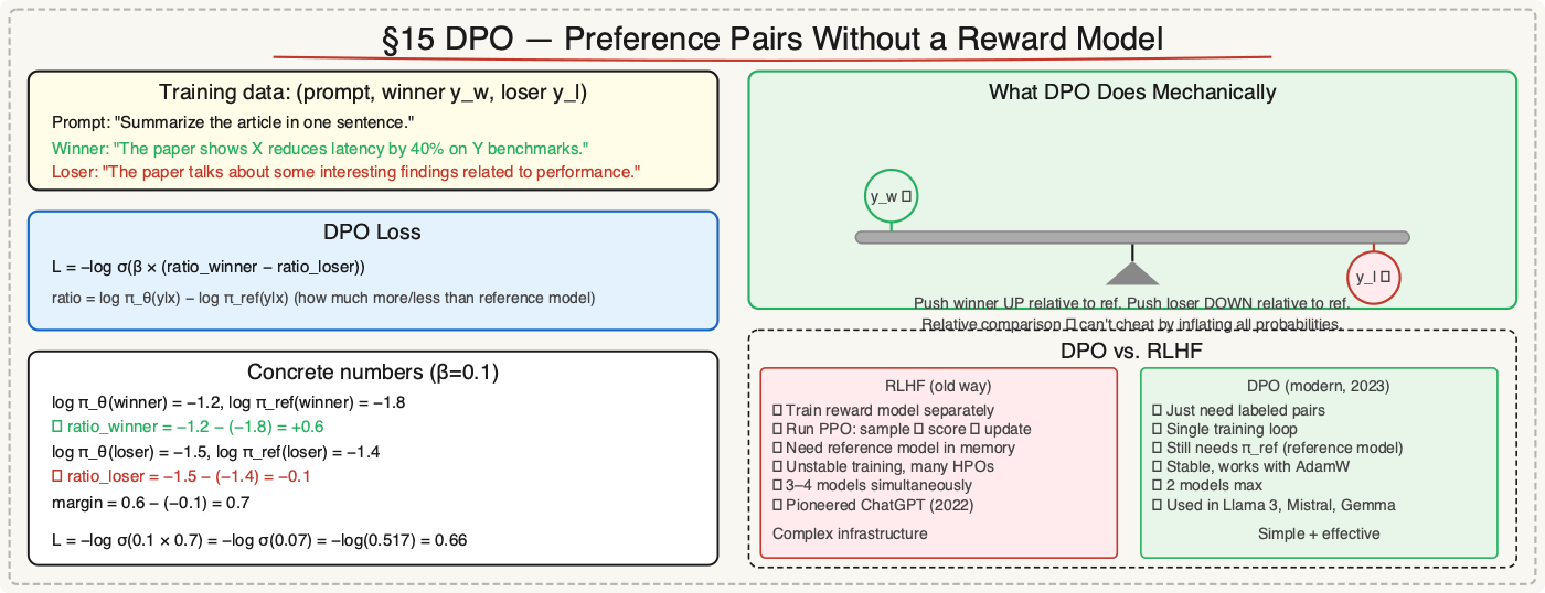
SFT teaches the model how to answer. But it doesn't teach quality. DPO trains the model to prefer human-chosen responses over rejected ones, without a separate reward model.
The DPO loss:
That's a mouthful. Break it down:
π_θ= the model we're trainingπ_ref= the base SFT model (frozen)y_w= the winning (preferred) responsey_l= the losing (rejected) responseβ= temperature controlling how strongly to diverge fromπ_ref(typically 0.1–0.5)σ= sigmoid function
What it does in plain terms:
For each pair (prompt, winner, loser):

ratio_winner = log π_θ(winner|prompt) − log π_ref(winner|prompt)
ratio_loser  = log π_θ(loser|prompt)  − log π_ref(loser|prompt)

L = −log σ(β × (ratio_winner − ratio_loser))
The model is rewarded for increasing the winner's probability relative to the reference model more than it increases the loser's. It's a relative comparison, not an absolute score — so the model can't just inflate all probabilities.
Concrete example:
Prompt: "Summarize the article in one sentence."
Winner: "The paper shows X reduces latency by 40% on Y benchmarks."
Loser:  "The paper talks about some interesting findings related to performance."

log π_θ(winner) = −1.2  →  log π_ref(winner) = −1.8  →  ratio_winner = +0.6
log π_θ(loser)  = −1.5  →  log π_ref(loser)  = −1.4  →  ratio_loser  = −0.1

margin = 0.6 − (−0.1) = 0.7
L = −log σ(0.1 × 0.7) = −log σ(0.07) = −log(0.517) = 0.66
Gradient flows: push up winner probability, push down loser probability, stay close to π_ref. That's the whole mechanism.
DPO exists because the alternative is heavy: a separate reward model plus a PPO loop. If you want to see exactly what it replaces, the build post implements that full pipeline — Phase 7 (reward model) and Phase 8 (PPO with KL penalty) — in runnable PyTorch.
16. Fine-Tuning: RLVR (Reinforcement Learning from Verifiable Rewards)
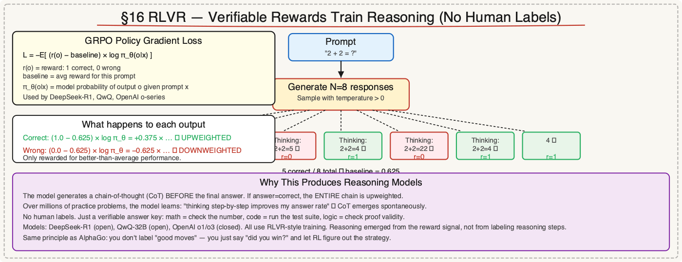
For math and code, you don't need human preference pairs. You can check if the answer is correct automatically.
The RLVR setup:
1. Model generates N candidate responses (e.g. N=8)
2. Each response is scored: r = 1 if answer correct, 0 if wrong
3. Policy gradient update: nudge the model toward responses that got r=1
The policy gradient loss (GRPO variant, used by DeepSeek-R1):
Where: - o = one generated output - r(o) = reward (1 or 0 for correct/wrong) - baseline = average reward across the N outputs for this prompt (reduces variance) - π_θ(o|x) = probability the model assigns to generating output o
Why baseline matters:
Prompt: "2 + 2 = ?"
8 outputs: 5 correct (r=1), 3 wrong (r=0)
baseline = 5/8 = 0.625

For a correct output:   (1.0 − 0.625) × log π_θ(o) = +0.375 × (...)  ← upweighted
For a wrong output:     (0.0 − 0.625) × log π_θ(o) = −0.625 × (...)  ← downweighted
The model only gets rewarded for doing better than its own average — this prevents it from gaming the reward by just being confidently wrong.
This is what powers reasoning models (DeepSeek-R1, QwQ, o3). The model generates a chain-of-thought, the final answer is checked, and the entire chain is upweighted or downweighted. Over millions of practice problems, it learns to think before answering. No human label — just a correct answer key.
17. KV Cache
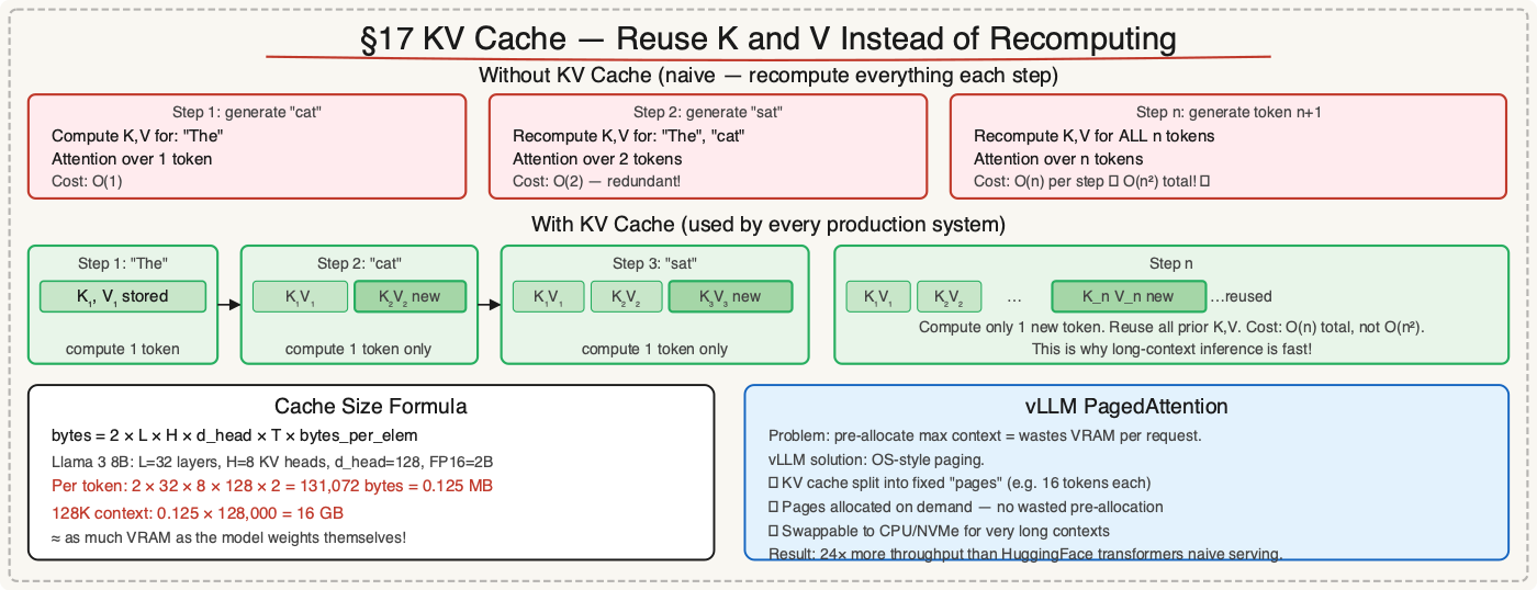
During inference, attention needs K and V vectors for every previous token. Without caching, predicting token 1000 would require recomputing K, V for tokens 1–999 from scratch — 999 full forward passes.
The KV cache stores K and V as they're computed, and reuses them:
Step 1: Compute and store K₁, V₁ for "The"
Step 2: Compute K₂, V₂ for "cat";   attention uses [K₁,K₂], [V₁,V₂]
Step 3: Compute K₃, V₃ for "sat";   attention uses [K₁,K₂,K₃], [V₁,V₂,V₃]
Step n: Compute Kₙ, Vₙ only;        attention reuses all prior K,V
Cache size formula:
For Llama 3 8B (32 layers, 8 KV heads, d_head=128, FP16 = 2 bytes):
Per token: 2 × 32 × 8 × 128 × 2 = 131,072 bytes = 0.125 MB
128K context (Llama 3.1+): 0.125 × 128,000 = 16 GB — as much as the model weights
This is why long contexts cost more — the KV cache is a second copy of memory that scales linearly with context length. vLLM's PagedAttention treats this like OS paging: allocating KV cache in blocks and swapping to CPU/disk, enabling much longer contexts on the same GPU.
A KV cache is also easy to get silently wrong — it generates garbage without ever crashing. The build post has a working KVCache class plus the 4-line equivalence test that catches a broken one (cached decode must match the full forward pass to ~1e-6).
18. Quantization
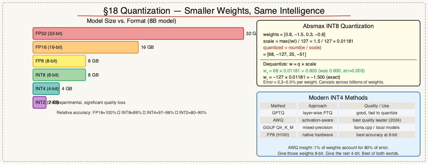
Model weights are stored as floating-point numbers. The more bits, the more precision — and memory.
FP32 (32-bit): each weight = 4 bytes → 8B model = 32 GB
FP16 (16-bit): each weight = 2 bytes → 8B model = 16 GB
INT8  (8-bit): each weight = 1 byte  → 8B model =  8 GB
INT4  (4-bit): each weight = 0.5 bytes → 8B model = 4 GB
Absmax quantization maps a float to INT8:
scale = max(|w|) / 127
w_quantized = round(w / scale)

Example: weights = [0.8, -1.5, 0.3, -0.6], max(|w|) = 1.5
scale = 1.5 / 127 = 0.01181

Quantized: [68, -127, 25, -51]
To dequantize (recover approximate original): w ≈ w_quantized × scale
w_0 = 68 × 0.01181 = 0.803   (was 0.800, error = 0.003)
w_1 = −127 × 0.01181 = −1.500 (exact)
w_2 = 25 × 0.01181 = 0.295   (was 0.300, error = 0.005)
The error is small — rounding to 256 levels introduces about 0.3–0.5% relative error per weight. Across billions of weights, errors partially cancel out, and benchmarks show INT4 models typically lose only 1–3% accuracy vs. FP16.
| Format | Bits | 8B model size | Where you'll see it |
|---|---|---|---|
| FP16 | 16 | 16 GB | Training, high-precision serving |
| FP8 | 8 | 8 GB | H100/H200 GPU inference |
| INT8 | 8 | 8 GB | bitsandbytes, llama.cpp Q8 |
| INT4 | 4 | 4 GB | AWQ, GPTQ, GGUF Q4_K_M |
| INT2 | 2 | 2 GB | Experimental, significant quality loss |
AWQ (Activation-Aware Weight Quantization) is the current quality leader for 4-bit: it identifies which weights matter most (based on activation scale) and gives them higher precision, rather than quantizing everything equally.
Check the Math Yourself
Don't take this article's word for it. The entire Section 4 attention computation is 15 lines of NumPy:
import numpy as np

X = np.array([[1.0, 0.0, 0.5, 0.2],    # "The"
              [0.5, 1.0, 0.2, 0.8],    # " cat"
              [0.2, 0.5, 1.0, 0.3]])   # " sat"

W_Q = np.array([[0,1,0,0],[1,0,0,0],[0,0,0,1],[0,0,1,0]], dtype=float)
Q, K, V = X @ W_Q, X, X                  # W_K = W_V = I

scores = Q @ K.T / np.sqrt(4)            # scale by √d_k
mask = np.triu(np.full((3,3), -np.inf), k=1)   # causal mask
weights = np.exp(scores + mask)
weights /= weights.sum(axis=1, keepdims=True)  # softmax

print(weights[2].round(2))        # [0.31 0.39 0.3 ]  ← "sat" attention weights
print((weights @ V)[2].round(3))  # [0.564 0.54  0.534 0.464]
The output matches Section 4 to within ±0.001 — the article rounds the attention weights to 2 decimals before the weighted sum, NumPy doesn't. That tiny gap is itself a lesson: every printed number in an ML paper hides a rounding decision.
Three exercises that will teach you more than rereading:
- Change
W_Qto the identity matrix. Watch which token "sat" attends to most now, and explain why. - Remove the causal mask. Check what "The" can suddenly see.
- Recompute Section 9's logits with
X_final = [0.71, 0.63, 0.58, 0.52]and the 6-rowEfrom Section 2 — one matrix multiply:E @ x_final.
Summary
One forward pass, traced all the way through:
| Step | Operation | Input | Output |
|---|---|---|---|
| 1 | Tokenize | "The cat sat" | [976, 9059, 10139] |
| 2 | Embed | token IDs | X ∈ ℝ^(3×4) |
| 3 | RoPE | X | X with position baked in |
| 4–5 | Attention | X + W_Q,W_K,W_V | context-aware X ∈ ℝ^(3×4) |
| 6 | FFN | per-token vector | knowledge-enriched vector |
| 7 | LayerNorm | any vector | zero-mean, unit-variance vector |
| 8 | Block × L | block input | refined representations |
| 9 | Logits + softmax | final hidden state | probability over vocab |
| 10 | Cross-entropy | P(correct) = 0.147 | loss = 1.917 |
| 11 | Backprop | loss | ∂L/∂w for every weight |
| 12 | AdamW | gradients + momentum | updated weights |
| 13 | Pretraining | 15T tokens | base model |
| 14 | SFT | (prompt, response) pairs + LoRA | instruction-following model |
| 15 | DPO | (prompt, winner, loser) pairs | quality-tuned model |
| 16 | RLVR | verifiable answers + GRPO | reasoning model |
| 17 | KV cache | computed K, V | reused at each decode step |
| 18 | Quantization | FP16 weights | INT4 (4× smaller, ~2% quality loss) |
The one rule of thumb: every weight in the model exists because backpropagation found it useful for predicting the next token across some slice of the training data. Fine-tuning reuses the same mechanism — just with different data and loss objectives — to shape which next tokens the model finds useful to predict.
Go to the Source
Every technique in this post comes from a specific paper. Read them in this order and each one will already feel familiar:
| Section | Technique | Paper |
|---|---|---|
| 4–5 | Transformer attention | Attention Is All You Need (Vaswani et al., 2017) |
| 3 | RoPE | RoFormer (Su et al., 2021) |
| 5 | GQA | GQA: Training Generalized Multi-Query Transformer Models (Ainslie et al., 2023) |
| 13 | Chinchilla scaling | Training Compute-Optimal LLMs (Hoffmann et al., 2022) |
| 14 | LoRA | LoRA: Low-Rank Adaptation (Hu et al., 2021) |
| 15 | DPO | Direct Preference Optimization (Rafailov et al., 2023) |
| 16 | GRPO / RLVR | DeepSeekMath (Shao et al., 2024) · DeepSeek-R1 (2025) |
| 17 | PagedAttention | Efficient Memory Management for LLM Serving (Kwon et al., 2023) |
| 18 | AWQ | AWQ: Activation-aware Weight Quantization (Lin et al., 2023) |
Ready to build it? Building an LLM from Scratch in PyTorch turns every section of this post into verified, runnable code — including a real training run you can reproduce in 7 minutes on a CPU.
Questions or discussion? Connect on LinkedIn, X or reach out via email.
Discussion
Have thoughts on this post? Share them below — questions, corrections, or your own experience are all welcome.